Simulation
This example demonstrates how to generate simulation plots from raw data as presented in the manuscript. In manuscript, we considered three simulation cases examining \(\mu\), \(\tau^2\), and \(\sigma_0^2\), along with two distribution variants: Gamma and Student’s \(t\) distributions. Below, we focus on the case of \(\mu\).
Generating simulation data
To generate the raw simulation data, we run the simulation script SIMU_MU.R, First, we import the required packages and configure the test values for \(\mu\):
library(BIT)
library(truncdist)

# Configuration parameters ---------------------------------------------------
TR_SIZES <- c(500, 1000, 1500)
MU_VALUES <- c(-5, -4.5, -4, -3.5, -3, -2.5)
TAU_SQ_VALUES <- c(0.5, 0.7, 0.9, 1.1, 1.3, 1.5)
SIGMA0_VALUES <- c(1, 1.2, 1.4, 1.6, 1.8, 2.0)
BASE_DIR <- "./simulation/MU"
N_VALUE <- 30000
ITERATIONS <- 5000
BURN_IN <- 2500
Next, we define helper functions used to generate simulation data for TRs with either single or multiple observations (datasets):
# Helper functions --------------------------------------------------------
logistic_transform <- function(theta) {
  exp(theta) / (1 + exp(theta))
}

generate_TR_size <- function(num_TRs) {
  ceiling(rtrunc(num_TRs, spec = "lnorm",
                 meanlog = 1, sdlog = 1.75,
                 a = 0, b = 1000))
}

generate_multi_obs_TR <- function(n, mu, tau_sq, population) {
  TR_data <- list()
  TR_data$theta_i <- rnorm(1, mu, sqrt(tau_sq))
  TR_data$sigma_i <- rgamma(1, 0.75, 100)
  TR_data$theta_ij <- rnorm(n, TR_data$theta_i, sqrt(TR_data$sigma_i))
  TR_data$x_ij <- rbinom(n, population, logistic_transform(TR_data$theta_ij))
  TR_data$n_ij <- rep(population, n)
  TR_data
}

generate_single_obs_TR <- function(mu, tau_sq, sigma0_sq, population) {
  TR_data <- list()
  TR_data$theta_i <- rnorm(1, mu, sqrt(tau_sq))
  TR_data$theta_ij <- rnorm(1, TR_data$theta_i, sqrt(sigma0_sq))
  TR_data$x_ij <- rbinom(1, population, logistic_transform(TR_data$theta_ij))
  TR_data$n_ij <- population
  TR_data
}
With these helper functions in place, we define the main function for generating simulation data:
# Data generation functions -----------------------------------------------
generate_simulation_data <- function(
    num_TRs = 1000,
    population = 30000,
    mu = -4,
    tau_sq = 0.75,
    sigma0_sq = 1.5) {

  TR_sizes <- generate_TR_size(num_TRs)

  multi_obs_count <- sum(TR_sizes > 1)
  single_obs_count <- num_TRs - multi_obs_count
  ordered_sizes <- sort(TR_sizes[TR_sizes > 1])

  simulation_data <- vector("list", num_TRs)

  # Generate multi-observation TRs
  for (i in seq_len(multi_obs_count)) {
    simulation_data[[i]] <- generate_multi_obs_TR(
      ordered_sizes[i], mu, tau_sq, population
    )
  }

  # Generate single-observation TRs
  for (j in (multi_obs_count + 1):num_TRs) {
    simulation_data[[j]] <- generate_single_obs_TR(
      mu, tau_sq, sigma0_sq, population
    )
  }

  simulation_data
}

structure_simulation_data <- function(raw_data) {
  structured_data <- list(
    xij = unlist(lapply(raw_data, `[[`, "x_ij")),
    nij = unlist(lapply(raw_data, `[[`, "n_ij")),
    label_vec = rep(seq_along(raw_data), lengths(lapply(raw_data, `[[`, "x_ij"))),
    theta_i = unlist(lapply(raw_data, `[[`, "theta_i")),
    theta_ij = unlist(lapply(raw_data, `[[`, "theta_ij"))
  )
  structured_data
}
The simulation workflow consists of generating the data, running the main analysis, and saving the results:
# Simulation workflow ----------------------------------------------------
run_simulation <- function(mu_value, iterations, num_TRs, simulation_id) {
  data_dir <- file.path(BASE_DIR, "SIMU_DATA")
  result_dir <- file.path(BASE_DIR, "SIMU_RESULTS")
  log_dir <- file.path(BASE_DIR, "LOG")

  dir.create(data_dir, showWarnings = FALSE, recursive = TRUE)
  dir.create(result_dir, showWarnings = FALSE, recursive = TRUE)
  dir.create(log_dir, showWarnings = FALSE, recursive = TRUE)

  # Generate and save simulation data
  simulated_data <- generate_simulation_data(
    num_TRs, N_VALUE, mu_value, 0.75, 1.5
  )
  structured_data <- structure_simulation_data(simulated_data)

  data_path <- file.path(data_dir, sprintf("id_%d_data_sim_mu_%g_I_%d.rds",
                                           simulation_id, mu_value, num_TRs))
  log_path <- file.path(log_dir, sprintf("id_%d_data_sim_mu_%g_I_%d.txt",
                                         simulation_id, mu_value, num_TRs))
  saveRDS(structured_data, data_path)

  # Run main analysis
  analysis_results <- Main_Sampling(
    iterations,
    structured_data$xij,
    structured_data$nij,
    structured_data$label_vec,
    log_path
  )

  # Process and save results
  final_results <- list(
    mu = mean(analysis_results$mu0[(iterations - BURN_IN):iterations]),
    theta_i = rowMeans(analysis_results$theta_i[, (iterations - BURN_IN):iterations]),
    label_vec = structured_data$label_vec
  )

  result_path <- file.path(result_dir, sprintf("id_%d_res_sim_mu_%g_I_%d.rds",
                                               simulation_id, mu_value, num_TRs))
  saveRDS(final_results, result_path)
}
We run the simulation 100 times for each setting, using different total numbers of TRs (500, 1000, and 1500), and varying \(\mu\) range from \([-5,-2.5]\), while keeping \(\tau^2=0.75\) and \(\sigma_0^2=1.5\) as default values.
# Execution block ------------------------------------------------------
for (mu_value in MU_VALUES){
  for (sim_id in seq_len(100)) {
    for (tr_size in TR_SIZES) {
      run_simulation(
        mu_value = mu_value,
        iterations = ITERATIONS,
        num_TRs = tr_size,
        simulation_id = sim_id
      )
    }
  }
}
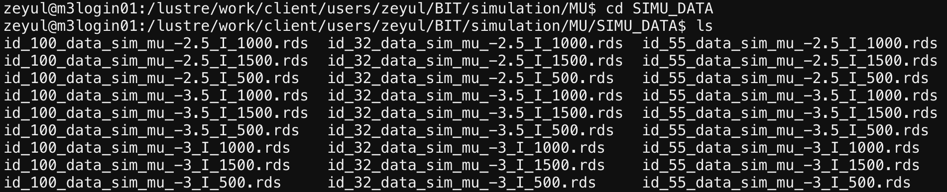
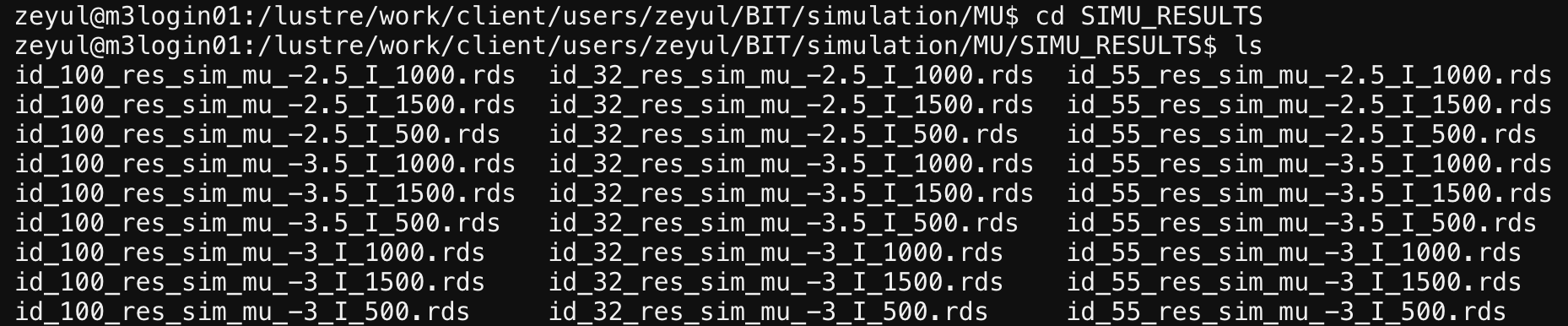
The simulation raw data and BIT derived results will be saved as *.rds files in two separate folders: ./simulation/MU/SIMU_DATA and ./simulation/MU/SIMU_RESULTS.
./simulation/MU/SIMU_DATA
./simulation/MU/SIMU_RESULTS
Next we need to calculate the mean squared error of \(\mu\) and spearman rho of estimated \(\hat{\theta}_i\) with true \(\theta_i\) from the raw data:
library(data.table)

logit_function<-function(x){
      return(log(x/(1-x)))
}

vec_logit<-Vectorize(logit_function)

Naive_Mu<-function(data){
  part1<-data$xij/data$nij
  part1[which(part1==0)]<-part1[which(part1==0)]+0.000001
  part1<-vec_logit(part1)
  group_means <- tapply(part1, data$label_vec, mean)
  return(mean(group_means))
}

Naive_TAU2<-function(data){
      part1<-data$xij/data$nij
      part1[which(part1==0)]<-part1[which(part1==0)]+0.000001
      part1<-vec_logit(part1)
      return(var(part1))
}

Naive_SIGMA0<-function(data,Mc){
      part1<-data$xij/data$nij
      part1[which(part1==0)]<-part1[which(part1==0)]+0.000001
      part1<-vec_logit(part1)
      Mu_est<-Naive_Mu(data)
      part1_Mc<-part1[(length(part1)-Mc+1):length(part1)]
      return(sum((part1_Mc-Mu_est)^2)/(Mc-1))
}

Naive_Theta_i<-function(data){
      part1<-data$xij/data$nij
      part1[which(part1==0)]<-part1[which(part1==0)]+0.000001
      part1<-vec_logit(part1)
      return(tapply(part1,data$label_vec,mean))
}


###################
work_dir_data<-"./simulation/MU/SIMU_DATA/"
work_dir_results<-"./simulation/MU/SIMU_RESULTS/"
output_dir<-"./simulation/RESULTS/MU/"
dir.create(output_dir, showWarnings = FALSE, recursive = TRUE))

M_vec<-c(350,700,1050)
Mc_vec<-c(150,300,450)
MU<-c(-5,-4.5,-4,-3.5,-3,-2.5)


for(i in 1:3){
              output_mu_df<-data.frame(matrix(nrow=6,ncol=4))
              colnames(output_mu_df)<-c("BIT_Bias","BIT_MSE","Naive_Bias","Naive_MSE")
              for(k in 1:6){
                      output_theta_i_df<-data.frame(matrix(nrow=(M_vec[i]+Mc_vec[i]),ncol=6))
                      colnames(output_theta_i_df)<-c("BIT_Bias","BIT_MSE","Naive_Bias","Naive_MSE","Naive_Spearman","BIT_Spearman")

                      data_files<-list.files(work_dir_data,pattern=paste0("*_mu_",MU[k],"_I_",M_vec[i]+Mc_vec[i],".rds"))
                      results_files<-list.files(work_dir_results,pattern=paste0("*_mu_",MU[k],"_I_",M_vec[i]+Mc_vec[i],".rds"))

                      naive_MU_vec<-c()
                      naive_Theta_mat<-matrix(nrow=(M_vec[i]+Mc_vec[i]),ncol=100)

                      BIT_MU_vec<-c()
                      BIT_Theta_mat<-matrix(nrow=(M_vec[i]+Mc_vec[i]),ncol=100)

                      for(m in 1:100){
                      print(paste0(i,"_",k,"_",m))
                              data<-readRDS(paste0(work_dir_data,data_files[m]))
                              results<-readRDS(paste0(work_dir_results,results_files[m]))

                              label_rank<-rank(-data$theta_i)

                              true_mu<-MU[k]
                              true_Theta_i<-data$theta_i

                              naive_Mu<-Naive_Mu(data)
                              naive_Theta_i<-Naive_Theta_i(data)

                              naive_rank<-rank(-naive_Theta_i)
                              names(naive_rank)<-NULL

                              BIT_Mu<-results$mu
                              BIT_Theta_i<-results$theta_i[!duplicated(results$label_vec)]

                              BIT_rank<-rank(-BIT_Theta_i)

                              naive_MU_vec<-c(naive_MU_vec,naive_Mu-true_mu)
                              BIT_MU_vec<-c(BIT_MU_vec,BIT_Mu-true_mu)

                              naive_Theta_mat[,m]<-naive_Theta_i-true_Theta_i
                              BIT_Theta_mat[,m]<-BIT_Theta_i-true_Theta_i

                              spearman_naive<-cor(label_rank,naive_rank,method="spearman")
                              spearman_BIT<-cor(label_rank,BIT_rank,method="spearman")

                              output_theta_i_df[m,5]<-spearman_naive
                              output_theta_i_df[m,6]<-spearman_BIT
                      }
                      output_mu_df[k,1]<-mean(abs(BIT_MU_vec),na.rm=TRUE)
                      output_mu_df[k,2]<-mean(BIT_MU_vec^2,na.rm=TRUE)
                      output_mu_df[k,3]<-mean(abs(naive_MU_vec),na.rm=TRUE)
                      output_mu_df[k,4]<-mean(naive_MU_vec^2,na.rm=TRUE)

                      output_theta_i_df[,1]<-rowMeans(abs(BIT_Theta_mat),na.rm=TRUE)
                      output_theta_i_df[,2]<-rowMeans(BIT_Theta_mat^2,na.rm=TRUE)
                      output_theta_i_df[,3]<-rowMeans(abs(naive_Theta_mat),na.rm=TRUE)
                      output_theta_i_df[,4]<-rowMeans(naive_Theta_mat^2,na.rm=TRUE)

                      fwrite(output_theta_i_df,paste0(output_dir,"Theta_i_I_",M_vec[i]+Mc_vec[i],"_Mu_",MU[k],".csv"))
              }
              fwrite(output_mu_df,paste0(output_dir,"Mu_I_",M_vec[i]+Mc_vec[i],".csv"))
}
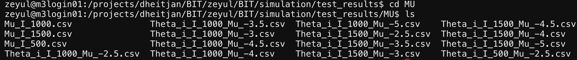
We will get tables as below:
./simulation/RESULTS/MU
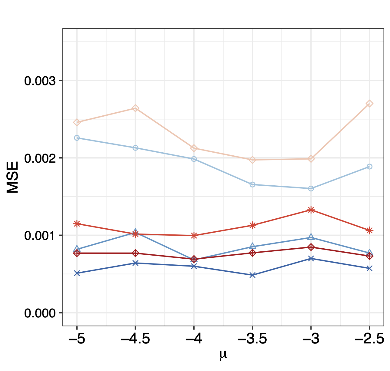
Generating Figure. 2A
We generate the Fig2A_Mu.csv table from the summarized results:
work_dir_MU<-"./simulation/RESULTS/MU/"
I_vec<-c(500,1000,1500)

new_df<-data.frame(matrix(nrow=6,ncol=7))
colnames(new_df)[1]<-"mu"
new_df[,1]<-c(-5.0,-4.5,-4,-3.5,-3,-2.5)
for(i in 1:3){
  data_df<-read.csv(paste0(work_dir_MU,"Mu_I_",I_vec[i],".csv"))
  new_df[,i+1]<-data_df$BIT_MSE[c(1,2,3,4,5,6)]
  new_df[,3+i+1]<-data_df$Naive_MSE[c(1,2,3,4,5,6)]
}

colnames(new_df)<-c("MU","BIT500","BIT1000","BIT1500","Naive500","Naive1000","Naive1500")
write.csv(new_df,"./simulation/RESULTS/Fig2A_MU.csv",row.names=FALSE)
The Fig2A_MU.csv table should be:
MU |
BIT500 |
BIT1000 |
BIT1500 |
Naive500 |
Naive1000 |
Naive1500 |
|
|---|---|---|---|---|---|---|---|
1 |
-5 |
0.0022580188135531 |
0.000818472327772802 |
0.000510569741043017 |
0.00245874128916261 |
0.00114969905279038 |
0.000769359289984737 |
2 |
-4.5 |
0.00212966515481292 |
0.00103666958740791 |
0.00064169937082568 |
0.00264156021151374 |
0.00101536653110342 |
0.000768920849747399 |
3 |
-4 |
0.00198518372879334 |
0.000681825887143333 |
0.000600056078685824 |
0.00212557745481653 |
0.000996199499101249 |
0.000692048219199762 |
4 |
-3.5 |
0.00165538478428067 |
0.000852297662144227 |
0.000485813251788291 |
0.00197356914261532 |
0.00112894933573882 |
0.000772942245152072 |
5 |
-3 |
0.00160390407139712 |
0.000971558635515894 |
0.000700264757159971 |
0.00198764288931968 |
0.00132907774386411 |
0.000847521525906551 |
6 |
-2.5 |
0.00188736351670382 |
0.000770553000802977 |
0.000572850943985385 |
0.00270199537402184 |
0.0010627703005949 |
0.000731624494748081 |
With the Fig2A_MU.csv table, we can now plot the MSE of BIT and naive methods:
MU_sim<-read.csv("./simulation/RESULTS/Fig2A_MU.csv")
long_data_mu <- pivot_longer(MU_sim, cols = -MU, names_to = "variable", values_to = "value")

p1<-ggplot(long_data_mu, aes(x = MU, y = value, color = variable, shape = variable)) +
  geom_line() +     # Add lines
  geom_point() +    # Add points
  scale_color_manual(values = c("BIT500" = colors_element1[1], "BIT1000" = colors_element1[2], "BIT1500" = colors_element1[3],"Naive500" = colors_element2[1], "Naive1000" = colors_element2[2], "Naive1500" = colors_element2[3]),
                     labels = c("BIT500" = "BIT (I=500)", "BIT1000" = "BIT (I=1000)", "BIT1500" = "BIT (I=1500)","Naive500" = "Naïve (I=500)", "Naive1000" = "Naïve (I=1000)", "Naive1500" = "Naïve (I=1500)"), name = "") +
  scale_shape_manual(values = c("BIT500" = 1, "BIT1000" = 2, "BIT1500" = 4,"Naive500" = 5, "Naive1000" = 8, "Naive1500" = 9),
                     labels = c("BIT500" = "BIT (I=500)", "BIT1000" = "BIT (I=1000)", "BIT1500" = "BIT (I=1500)","Naive500" = "Naïve (I=500)", "Naive1000" = "Naïve (I=1000)", "Naive1500" = "Naïve (I=1500)"),name = "") +
  labs(title = "", x = expression(bold(mu)), y = "MSE") +
  theme_bw() + theme(legend.position = "none",axis.text.x = element_text(size = 12,color="black"),  # Customizing x-axis tick labels
                     axis.text.y = element_text(size = 10,color="black"),  # Customizing y-axis tick labels
                     axis.title.x = element_text(size = 12,color="black"), # Customizing x-axis label
                     axis.title.y = element_text( size = 12,color="black"), # Customizing y-axis label
                     legend.text = element_text(size = 10,color="black"),  # Customizing legend text
                     legend.title = element_text( size = 12,color="black")  # Customizing legend title
  ) + scale_x_continuous(labels=c("-5","-4.5","-4","-3.5","-3","-2.5"))+scale_y_continuous(limits=c(0,0.0035),breaks=c(0,0.0010,0.0020,0.0030))
Which gives us:
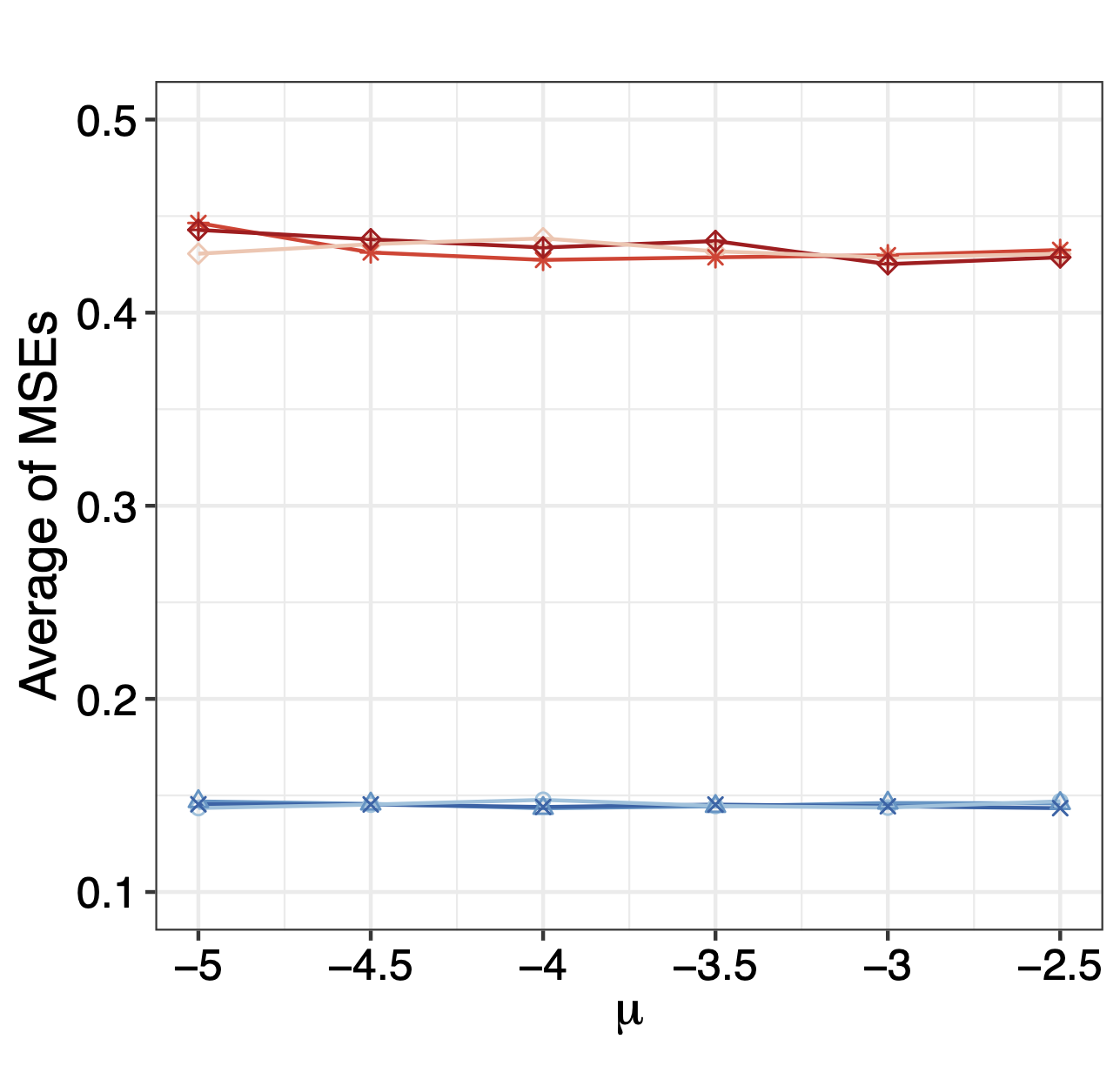
Generating Figure. 2B
We generate the Fig2B_MU.csv table from the summarized results:
library(tidyverse)
work_dir_MU<-"./simulation/RESULTS/MU/"

I_vec<-c(500,1000,1500)
mu<-c(-5,-4.5,-4,-3.5,-3,-2.5)
THETA_MSE_MU<-data.frame(matrix(nrow=18,ncol=4))
colnames(THETA_MSE_MU)<-c("MU","I_SIZE","BIT_MSE_MEAN","Naive_MSE_MEAN")
THETA_MSE_MU$MU<-rep(mu,3)
THETA_MSE_MU$I_SIZE<-rep(I_vec,each=6)

for(i in 1:3){
  BIT_MSE_Mean<-c()
  Naive_MSE_Mean<-c()

  for(k in 1:6){
    data_df<-read.csv(paste0(work_dir_MU,"Theta_i_I_",I_vec[i],"_Mu_",mu[k],".csv"))
    BIT_MSE_Mean<-c(BIT_MSE_Mean,mean(data_df[,2],na.rm=TRUE))
    Naive_MSE_Mean<-c(Naive_MSE_Mean,mean(data_df[,4],na.rm=TRUE))
  }
  THETA_MSE_MU$BIT_MSE_MEAN[((1:6)+(i-1)*6)]<-BIT_MSE_Mean
  THETA_MSE_MU$Naive_MSE_MEAN[((1:6)+(i-1)*6)]<-Naive_MSE_Mean
}

THETA_MSE_MU <- THETA_MSE_MU %>%
    # Pivot the MSE columns to long format
    pivot_longer(
      cols = c(BIT_MSE_MEAN, Naive_MSE_MEAN),
      names_to = "method",
      values_to = "value"
    ) %>%
    # Create the group column by combining method and I_SIZE
    mutate(
      # Extract just "BIT" or "Naive" from the method names
      method = str_replace(method, "_MSE_MEAN", ""),
      # Create the group label in the desired format
      group = sprintf("%s (I=%d)", method, I_SIZE),
      # Rename mu column to match desired output
      mu = MU
    ) %>%
    # Select and arrange the final columns
    select(value, mu, group) %>%
    # Sort by mu and group
    arrange(mu, group)

write.csv(THETA_MSE_MU,"./simulation/RESULTS/Fig2B_MU.csv",row.names = FALSE)
The Fig2B_MU.csv table should be:
With the Fig2B_MU.csv table, we can now plot the MSE of BIT and naive methods:
Theta_MU_sim<-read.csv("./simulation/RESULTS/Fig2B_MU.csv")
plot1<-ggplot(Theta_MU_sim, aes(x = mu, y = value, color = group, shape = group)) +
  geom_line() +     # Add lines
  geom_point() +    # Add points
  scale_color_manual(values = c("BIT (I=500)" = colors_element1[1], "BIT (I=1000)" = colors_element1[2], "BIT (I=1500)" = colors_element1[3],"Naive (I=500)" = colors_element2[1], "Naive (I=1000)" = colors_element2[2], "Naive (I=1500)" = colors_element2[3]), name = "") +
  scale_shape_manual(values = c("BIT (I=500)" = 1, "BIT (I=1000)" = 2, "BIT (I=1500)" = 4,"Naive (I=500)" = 5, "Naive (I=1000)" = 8, "Naive (I=1500)" = 9),name = "") +
  labs(title = "", x = expression(bold(mu)), y = "Average of MSEs") +
  theme_bw() + theme(legend.position = "none",axis.text.x = element_text(size = 12,color="black"),  # Customizing x-axis tick labels
                     axis.text.y = element_text(size = 12,color="black"),  # Customizing y-axis tick labels
                     axis.title.x = element_text(size = 14,color="black"), # Customizing x-axis label
                     axis.title.y = element_text( size = 14,color="black"), # Customizing y-axis label
                     legend.text = element_text(size = 10,color="black"),  # Customizing legend text
                     legend.title = element_text( size = 12,color="black")  # Customizing legend title
  ) + scale_x_continuous(labels=c("-5","-4.5","-4","-3.5","-3","-2.5"))+scale_y_continuous(limits=c(0.1,0.5),breaks=c(0.1,0.2,0.3,0.4,0.5))
which gives the plot:
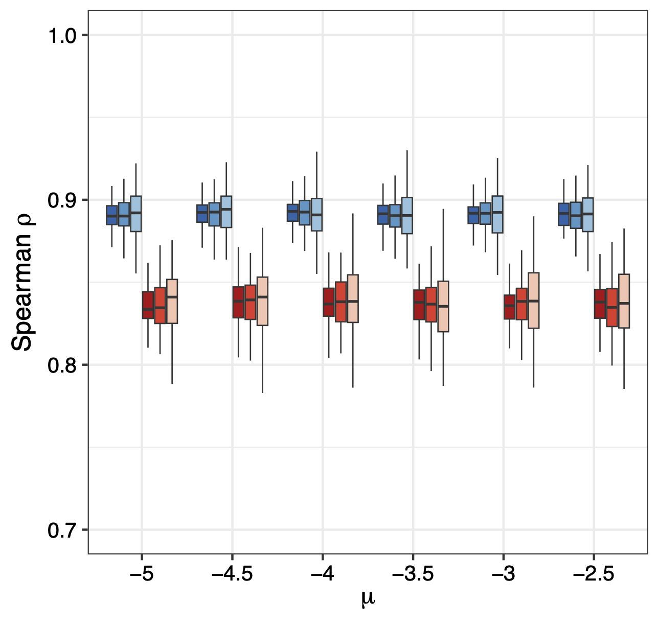
Generating Figure. 2C
We can also generate the Fig2C_MU.csv table:
work_dir_MU<-"./simulation/RESULTS/MU/"
work_files_MU<-list.files(work_dir_MU,pattern="Theta_i_I_*")
work_files_MU
I_vec<-c(500,1000,1500)
TR_level<-c("500","1000","1500")

mu<-c(-5,-4.5,-4,-3.5,-3,-2.5)
MU_spearman_df<-data.frame(matrix(nrow=3600,ncol=3))
colnames(MU_spearman_df)<-c("value","mu","group")
for(i in 1:6){
  for(j in 1:3){
    Theta_df<-as.data.frame(fread(paste0(work_dir_MU,"Theta_i_I_",I_vec[j],"_Mu_",mu[i],".csv")))
    index1<-(i-1)*600+(j-1)*200+1
    index2<-(i-1)*600+(j-1)*200+100
    index3<-(i-1)*600+(j-1)*200+101
    index4<-(i-1)*600+(j-1)*200+200
    MU_spearman_df[index1:index2,1]<-Theta_df$Naive_Spearman[1:100]
    MU_spearman_df[index3:index4,1]<-Theta_df$BIT_Spearman[1:100]
    MU_spearman_df[index1:index2,2]<-mu[i]
    MU_spearman_df[index3:index4,2]<-mu[i]
    MU_spearman_df[index1:index2,3]<-paste0("Naive (I=",TR_level[j],")")
    MU_spearman_df[index3:index4,3]<-paste0("BIT (I=",TR_level[j],")")
  }
}

df1<-MU_spearman_df
df1$mu<-as.factor(df1$mu)
df1$group<-factor(df1$group,levels=c("BIT (I=1500)","BIT (I=1000)","BIT (I=500)","Naive (I=1500)","Naive (I=1000)","Naive (I=500)"))

write.csv(df1,"./simulation/RESULTS/Fig2C_MU.csv",row.names=FALSE)
The Fig2C_MU.csv table should be:
With the Fig2C_MU.csv table, we can now plot the MSE of BIT and naive methods:
df1<-read.csv(paste0(DATA_DIR,"Fig2C_MU.csv"))
df1$mu<-as.factor(df1$mu)
df1$group<-factor(df1$group,levels=c("BIT (I=1500)","BIT (I=1000)","BIT (I=500)","Naive (I=1500)","Naive (I=1000)","Naive (I=500)"))

plot1<-ggplot(df1, aes(x = mu, y = value, fill = group)) +
  geom_boxplot(width = 0.7, size = 0.3,position = position_dodge(0.8), outlier.shape=NA)+
  ylim(c(0.7,1))+theme_bw()+theme(legend.position = "none",axis.text.x = element_text(size = 10,color="black"),  # Customizing x-axis tick labels
                                   axis.text.y = element_text( size = 10,color="black"),  # Customizing y-axis tick labels
                                   axis.title.x = element_text( size = 12,color="black"), # Customizing x-axis label
                                   axis.title.y = element_text( size = 12,color="black"), # Customizing y-axis label
                                   legend.text = element_text( size = 8,color="black"),  # Customizing legend text
                                   legend.title = element_text(size = 10,color="black")  # Customizing legend title
  )+
  scale_fill_manual(values = c(colors_element1[3:1], colors_element2[3:1]))+
  xlab(expression(mu))+ylab(expression(paste("Spearman ",rho)))
which gives the plot: