RUNX1 Plots
The following example demonstrates how to process raw ATAC-seq data obtained from the Sequence Read Archive (SRA). Specifically, the workflow includes data download, quality checking, trimming, alignment with Bowtie2, format conversion with Samtools, duplicate removal, and peak calling using MACS2. This complete pipeline ensures high-quality data preparation for generating BIT plots.
For illustration purposes, the pipeline below demonstrates processing for a single sample (RUNX1_WT_DN3_Rep1). However, in a complete analysis, three additional samples are required, including two replicates from knockout conditions and one additional replicate from the wild-type control.
#!/bin/bash
#SBATCH -J Fully_Process_Scripts_ATAC_seq
#SBATCH -o ./output/output-%j.out
#SBATCH -e ./error/error-%j.out
#SBATCH -p standard-s --mem=64G

# Change the directory as necessary
LOG_DIR="/lustre/work/client/users/zeyul/BIT/mm10/data/log/"
MM10_REF_DIR="/lustre/work/client/users/BIT/tools/mm10_ref_bowtie2/mm10"
DATA_DIR="/lustre/work/client/users/zeyul/BIT/mm10/data/"
FastQC_DIR="/lustre/work/client/users/zeyul/BIT/mm10/FastQC/"
PEAK_DIR="/lustre/work/client/users/zeyul/BIT/mm10/results/"
DiffBind_DIR="/lustre/work/client/users/zeyul/BIT/mm10/DiffBind/"

MIDDLE_DIR="RUNX1_KO/"

# Specific the final ATAC-seq filename and SRX number
ATAC_NAME_1="RUNX1_WT_Rep1"
SRX_NUMBER="SRR24493103"
#SRX_NUMBER="SRR24493101" WT Rep2
#SRX_NUMBER="SRR24493100" cKO Rep1
#SRX_NUMBER="SRR24493099" cKO Rep2

mkdir -p "${DATA_DIR}${MIDDLE_DIR}"
mkdir -p "${LOG_DIR}${MIDDLE_DIR}"
mkdir -p "${FastQC_DIR}${MIDDLE_DIR}"
mkdir -p "${PEAK_DIR}${MIDDLE_DIR}"

## Download Data
fasterq-dump --progress "$SRX_NUMBER" -o "${DATA_DIR}${MIDDLE_DIR}${ATAC_NAME_1}.fastq"

## FastQC before Trimming
fastqc --noextract --nogroup -o "${FastQC_DIR}${MIDDLE_DIR}" "${DATA_DIR}${MIDDLE_DIR}${ATAC_NAME_1}_1.fastq" "${DATA_DIR}${MIDDLE_DIR}${ATAC_NAME_1}_2.fastq"

## Trimming with trim-galore
trim_galore --paired -q 20 --phred33 --length 25 -e 0.1 --stringency 4 -o "${DATA_DIR}${MIDDLE_DIR}" "${DATA_DIR}${MIDDLE_DIR}${ATAC_NAME_1}_1.fastq" "${DATA_DIR}${MIDDLE_DIR}${ATAC_NAME_1}_2.fastq"
mkdir -p "${PEAK_DIR}${MIDDLE_DIR}"

## FastQC post-trimming
fastqc --noextract --nogroup -o "${FastQC_DIR}${MIDDLE_DIR}" "${DATA_DIR}${MIDDLE_DIR}${ATAC_NAME_1}_1_val_1.fq" "${DATA_DIR}${MIDDLE_DIR}${ATAC_NAME_1}_2_val_2.fq"

## bowtie2 Alignment
bowtie2 --very-sensitive -X 2000 -p 8 -q --local \
-x "${MM10_REF_DIR}" \
-1 "${DATA_DIR}${MIDDLE_DIR}${ATAC_NAME_1}_1_val_1.fq" -2 "${DATA_DIR}${MIDDLE_DIR}${ATAC_NAME_1}_2_val_2.fq" \
-S "${DATA_DIR}${MIDDLE_DIR}${ATAC_NAME_1}.sam"

## Samtools transfer to BAM
samtools view -h -S -b \
-o "${DATA_DIR}${MIDDLE_DIR}${ATAC_NAME_1}.bam" \
"${DATA_DIR}${MIDDLE_DIR}${ATAC_NAME_1}.sam"
samtools sort -n -o "${DATA_DIR}${MIDDLE_DIR}${ATAC_NAME_1}_sorted.bam" -O BAM "${DATA_DIR}${MIDDLE_DIR}${ATAC_NAME_1}.bam"
samtools fixmate -m "${DATA_DIR}${MIDDLE_DIR}${ATAC_NAME_1}_sorted.bam" "${DATA_DIR}${MIDDLE_DIR}${ATAC_NAME_1}_fixmate.bam"
rm "${DATA_DIR}${MIDDLE_DIR}${ATAC_NAME_1}_sorted.bam"
samtools sort -o "${DATA_DIR}${MIDDLE_DIR}${ATAC_NAME_1}_sorted.bam" "${DATA_DIR}${MIDDLE_DIR}${ATAC_NAME_1}_fixmate.bam"
samtools markdup -r -s "${DATA_DIR}${MIDDLE_DIR}${ATAC_NAME_1}_sorted.bam" "${DATA_DIR}${MIDDLE_DIR}${ATAC_NAME_1}_Final.bam"
samtools index "${DATA_DIR}${MIDDLE_DIR}${ATAC_NAME_1}_Final.bam"

samtools index "${DATA_DIR}${MIDDLE_DIR}${ATAC_NAME_1}_Final.bam"

## Peak Calling
macs2 callpeak -f BAM -g mm -n "${PEAK_DIR}${MIDDLE_DIR}${ATAC_NAME_1}" -B -q 0.01 -t "${DATA_DIR}${MIDDLE_DIR}${ATAC_NAME_1}_Final.bam"

# For DiffBind
mv "${DATA_DIR}${MIDDLE_DIR}${ATAC_NAME_1}_Final.bam" "${DATA_DIR}${MIDDLE_DIR}${ATAC_NAME_1}_peaks.narrowPeak" "${PEAK_DIR}${MIDDLE_DIR}"
The processed files need to be put in the same folder for the downstream DiffBind analysis
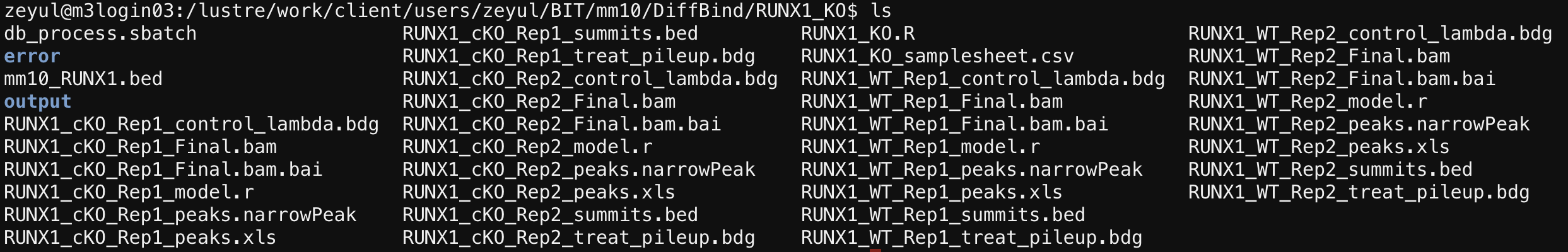
For DiffBind, we need to first formulate a samplesheet to list the datasets:
SampleID |
Factor |
Condition |
Treatment |
Replicate |
bamReads |
Peaks |
PeakCaller |
|
|---|---|---|---|---|---|---|---|---|
1 |
RUNX1_WT1 |
RUNX1 |
WT |
full |
1 |
RUNX1_WT_Rep1_Final.bam |
RUNX1_WT_Rep1_peaks.narrowPeak |
narrow |
2 |
RUNX1_WT2 |
RUNX1 |
WT |
full |
2 |
RUNX1_WT_Rep2_Final.bam |
RUNX1_WT_Rep2_peaks.narrowPeak |
narrow |
3 |
RUNX1_KO1 |
RUNX1 |
KO |
full |
1 |
RUNX1_cKO_Rep1_Final.bam |
RUNX1_cKO_Rep1_peaks.narrowPeak |
narrow |
4 |
RUNX1_KO2 |
RUNX1 |
KO |
full |
2 |
RUNX1_cKO_Rep2_Final.bam |
RUNX1_cKO_Rep2_peaks.narrowPeak |
narrow |
Next we need to use DiffBind to process and generate the differentially accessible region set.
library(DiffBind)
library(rtracklayer)

print(getwd())
samplesheet <- read.csv("RUNX1_KO_samplesheet.csv")
RUNX1_KO <- dba(sampleSheet = samplesheet)
RUNX1_KO <- dba.count(RUNX1_KO, minOverlap = 2)
RUNX1_KO <- dba.blacklist(RUNX1_KO, blacklist = DBA_BLACKLIST_MM10)
RUNX1_KO$config$cores = 64
RUNX1_KO$config$bUsePval = TRUE
RUNX1_KO$th = 0.20
RUNX1_KO_norm <- dba.normalize(RUNX1_KO, method = DBA_DESEQ2,
                               normalize = DBA_NORM_NATIVE,
                               library = DBA_LIBSIZE_BACKGROUND,
                               background = TRUE)
RUNX1_KO_ct <- dba.contrast(RUNX1_KO_norm, categories = DBA_CONDITION, minMembers = 2)
RUNX1_KO_results <- dba.analyze(RUNX1_KO_ct, method = DBA_DESEQ2)
RUNX1_KO <- dba.report(RUNX1_KO_results, file = "RUNX1_cKO_report.csv", th = 0.1)
export.bed(RUNX1_KO, "mm10_RUNX1.bed")
The exported BED file can be shown as:
# Load required library
library(rtracklayer)

# Define file path
RUNX1_BED <- "/Users/zeyulu/Desktop/Project/BIT/Input_Data/DARs/mm10_RUNX1.bed"

# Import BED file
import(RUNX1_BED)
Loading required package: GenomicRanges
Loading required package: GenomeInfoDb
Warning message:
package ‘GenomeInfoDb’ was built under R version 4.4.2

GRanges object with 15652 ranges and 2 metadata columns:
          seqnames              ranges strand |        name     score
             <Rle>           <IRanges>  <Rle> | <character> <numeric>
      [1]     chr3 143678121-143678521      * |       40711         0
      [2]    chr12   21480229-21480629      * |       12636         0
      [3]     chr1 192778787-192779187      * |        4468         0
      [4]    chr13     9547929-9548329      * |       15220         0
      [5]     chr7   88206431-88206831      * |       55040         0
      ...      ...                 ...    ... .         ...       ...
  [15648]     chr1   52799363-52799763      * |         796         0
  [15649]    chr14 105700293-105700693      * |       20509         0
  [15650]    chr12 111072186-111072586      * |       14669         0
  [15651]    chr16   93031654-93032366      * |       25272         0
  [15652]     chr4 117190116-117190516      * |       43363         0
  -------
  seqinfo: 24 sequences from an unspecified genome; no seqlengths
We next apply BIT to the exported BED file and generate the TR ranked table:
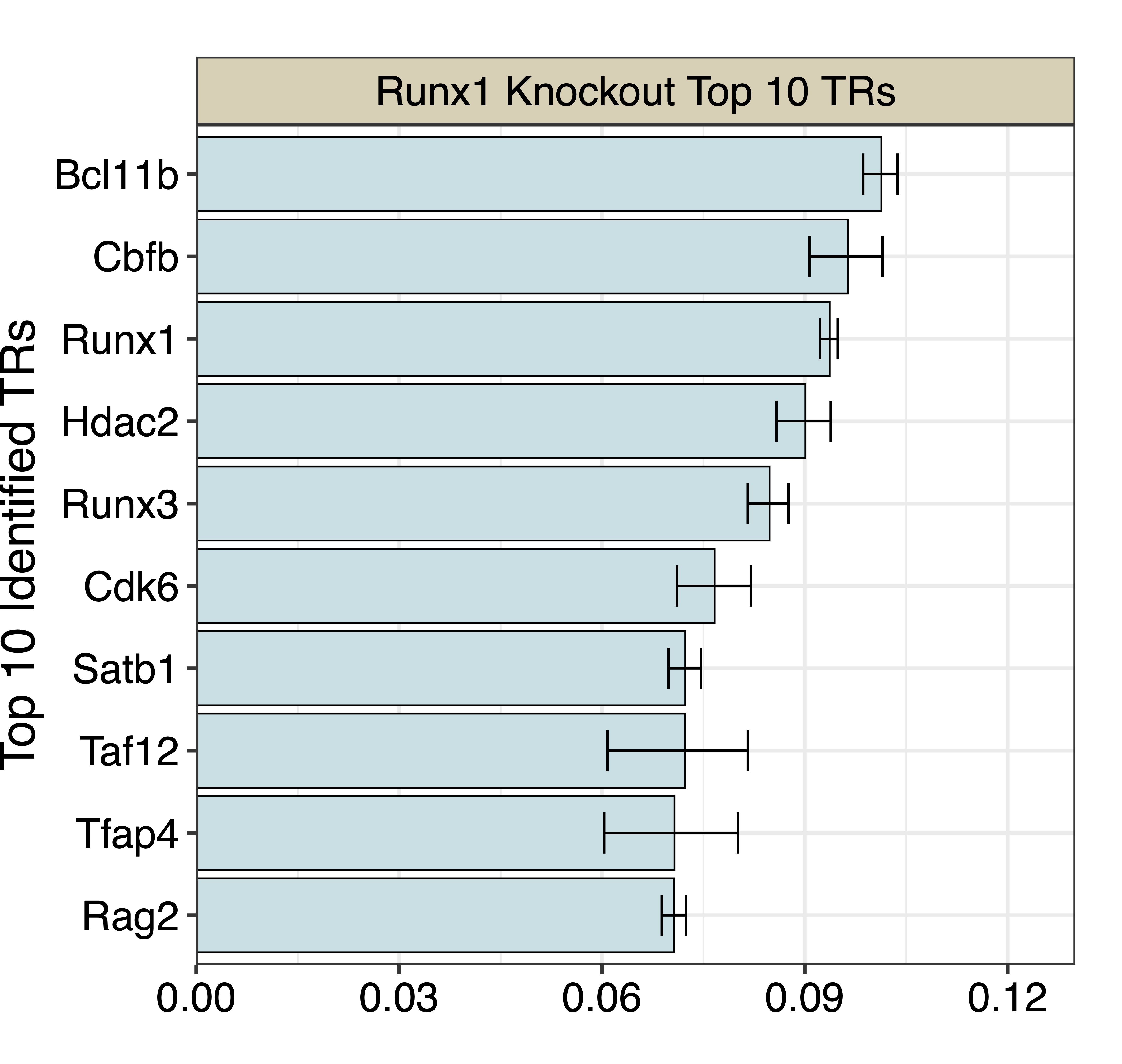
     TR   Theta_i     lower     upper  BIT_score BIT_score_lower BIT_score_upper Rank
 1  Bcl11b -2.182627 -2.212789 -2.156569 0.10132149      0.09860792      0.10371893    1
 2    Cbfb -2.238118 -2.305173 -2.180754 0.09637935      0.09069547      0.10149211    2
 3   Runx1 -2.269733 -2.286438 -2.255767 0.09366088      0.09225243      0.09485314    3
 4   Hdac2 -2.312496 -2.366128 -2.267778 0.09009334      0.08579231      0.09382692    4
 5   Runx3 -2.378822 -2.421391 -2.343063 0.08480192      0.08155599      0.08761877    5
 6    Cdk6 -2.488816 -2.570101 -2.415317 0.07664596      0.07108760      0.08201211    6
 7   Satb1 -2.551729 -2.589306 -2.517789 0.07231043      0.06982987      0.07462051    7
 8   Taf12 -2.552330 -2.737449 -2.421156 0.07227008      0.06079942      0.08157363    8
 9   Tfap4 -2.575503 -2.745504 -2.441114 0.07073173      0.06034110      0.08009081    9
10   Rag2 -2.576603 -2.604533 -2.550052 0.07065946      0.06884723      0.07242299   10
And we can plot the top 10 TRs:
# Load required libraries
library(ggplot2)

# Read the CSV file
RUNX1_Tab <- read.csv("/Users/zeyulu/Desktop/Project/BIT/revision_data/bin_width/1000/mm10_RUNX1_rank_table.csv", row.names = 1)

# Prepare data frame for visualization
data <- data.frame(
    Group = "Runx1 Knockout Top 10 TRs",
    Label = RUNX1_Tab[1:10, "TR"],
    Value = RUNX1_Tab[1:10, "BIT_score"],
    Upper = RUNX1_Tab[1:10, "BIT_score_upper"],
    Lower = RUNX1_Tab[1:10, "BIT_score_lower"]
)

# Convert Label to factor for ordering in the plot
data$Label <- factor(data$Label, levels = rev(data$Label))

# Create the plot using ggplot2
p1 <- ggplot(data, aes(x = Label, y = Value)) +
    geom_col(fill = "#C1E0E4", colour = "black", size = 0.25) +
    geom_errorbar(aes(ymin = Lower, ymax = Upper), width = 0.5, color = "black", size = 0.35) +
    coord_flip() +  # Flip coordinates for a horizontal bar plot
    facet_grid(. ~ Group, scales = "free_y") +  # Facet by group
    labs(title = "", x = "Top 10 Identified TRs", y = "") +
    scale_y_continuous(limits = c(0, 0.13), breaks = seq(0, 0.12, by = 0.03), expand = c(0, 0)) +
    theme_bw() +  # Minimal theme
    theme(
        axis.text.x = element_text(color = "black", size = 12),
        axis.text.y = element_text(color = "black", size = 12),
        axis.title.y = element_text(size = 14),
        legend.position = "none",
        plot.margin = unit(c(0, 0.5, 0, 0), "cm"),
        strip.background = element_rect(fill = "#DBD1B6"),
        strip.text = element_text(size = 12, colour = "black")
    )

# Display the plot
print(p1)
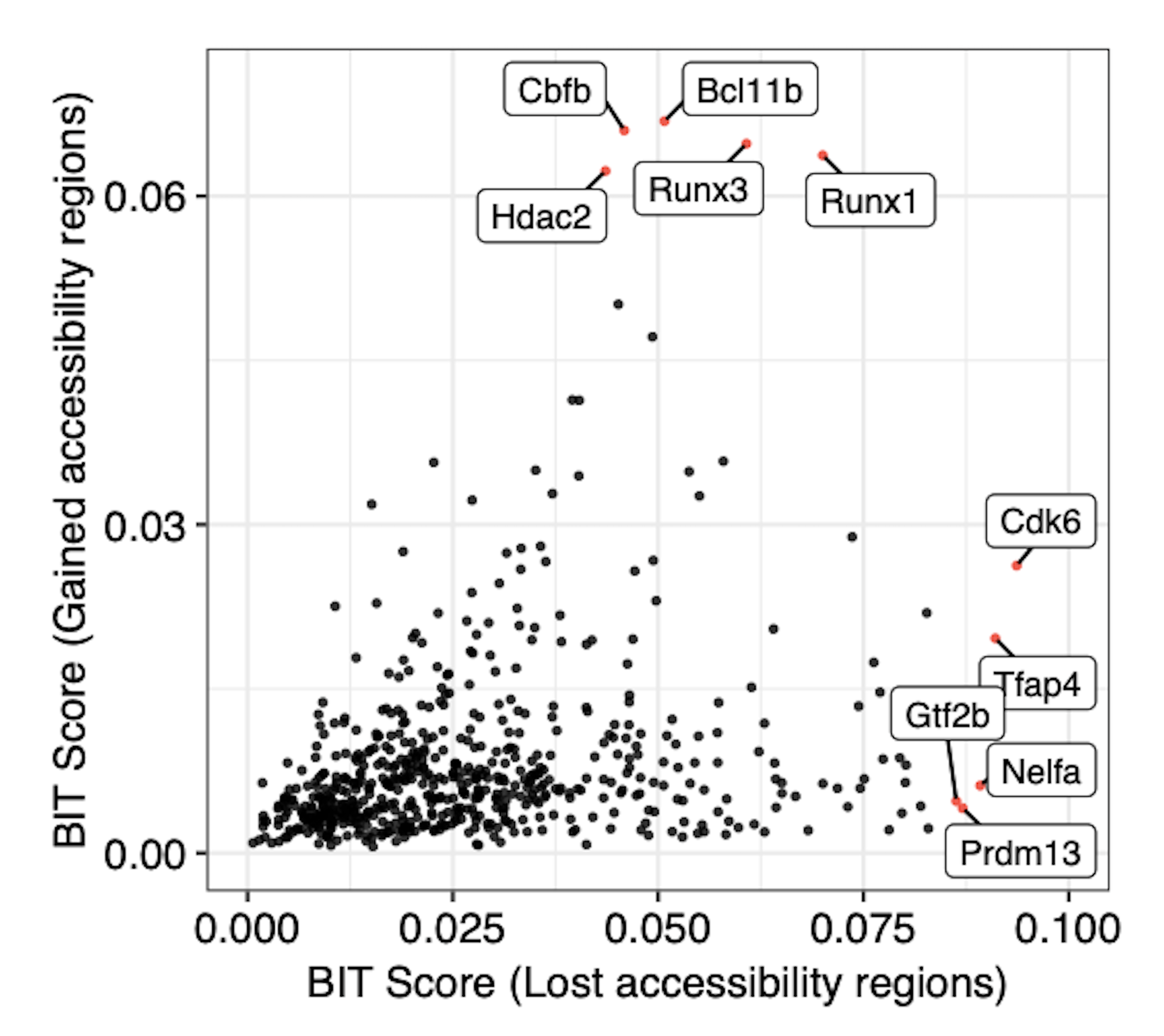
We can also generate the plot by comparing the BIT-identified TRs from using increased accessibility regions versus decreased accessibility regions. We separate the regions in the DiffBind generated report based on fold enrichment:
# Define file path
RUNX1_report <- "./test/RUNX1_cKO_report.csv"

# Read the CSV file
RUNX1_report_tab <- read.csv(RUNX1_report)

# Display the first six rows
head(RUNX1_report_tab)
           Chr     Start       End     Conc  Conc_KO  Conc_WT      Fold      p.value          FDR
1         chr3 143678121 143678521 7.277114 5.857603 7.978584 -1.986227 8.208806e-23 5.317866e-18
2        chr12  21480229  21480629 6.594209 4.497721 7.414836 -2.670207 1.638762e-22 5.317866e-18
3         chr1 192778787 192779187 7.073688 5.673339 7.770717 -1.954896 1.053971e-20 2.280126e-16
4        chr13   9547929   9548329 7.420042 6.200425 8.071361 -1.751839 1.479800e-20 2.401012e-16
5         chr7  88206431  88206831 7.940753 7.026219 8.496063 -1.409733 9.299981e-20 1.207156e-15
6 chrUn_JH584304     55478     55878 8.066727 7.232130 8.592054 -1.310974 1.948392e-19 2.107543e-15
We separate the table based on the fold enrichment change (Column: Fold)
# Load required library
library(dplyr)

# Separate rows based on the 'Fold' column
positive_fold <- RUNX1_report_tab %>%
  dplyr::filter(Fold > 0) %>%
  dplyr::select(Chr, Start, End)

negative_fold <- RUNX1_report_tab %>%
  dplyr::filter(Fold < 0) %>%
  dplyr::select(Chr, Start, End)

# Define output file paths
positive_bed_file <- "./test/RUNX1_KO_increased.bed"
negative_bed_file <- "./test/RUNX1_KO_decreased.bed"

# Export to .bed files without headers and row names
write.table(positive_fold, file = positive_bed_file, sep = "\t",
            row.names = FALSE, col.names = FALSE, quote = FALSE)

write.table(negative_fold, file = negative_bed_file, sep = "\t",
            row.names = FALSE, col.names = FALSE, quote = FALSE)

# Print messages for confirmation
cat("Positive fold BED file saved to:", positive_bed_file, "\n")
cat("Negative fold BED file saved to:", negative_bed_file, "\n")
# Load required library
library(rtracklayer)

# Import BED files
RUNX1_KO_increased <- import("./test/RUNX1_KO_increased.bed")
RUNX1_KO_decreased <- import("./test/RUNX1_KO_decreased.bed")

# Display summary of imported GRanges objects
RUNX1_KO_increased
RUNX1_KO_decreased
Console Output
After executing the script, the following output is displayed:
Increased RUNX1 Binding Regions:
 GRanges object with 4054 ranges and 0 metadata columns:
             seqnames              ranges strand
                <Rle>           <IRanges>  <Rle>
   [1] chrUn_JH584304         26924-27323      *
   [2]           chr2 105358113-105358512      *
   [3]           chr7   12987445-12987844      *
   [4]           chr3 126628458-126628857      *
   [5]           chr3 144260784-144261183      *
   ...            ...                 ...    ...
[4050]          chr15   83563327-83563726      *
[4051]           chr5 100070187-100070586      *
[4052]           chr5 122274739-122275138      *
[4053]          chr16   93031655-93032366      *
[4054]           chr4 117190117-117190516      *
-------
seqinfo: 21 sequences from an unspecified genome; no seqlengths
Decreased RUNX1 Binding Regions:
 GRanges object with 11598 ranges and 0 metadata columns:
        seqnames              ranges strand
           <Rle>           <IRanges>  <Rle>
    [1]     chr3 143678122-143678521      *
    [2]    chr12   21480230-21480629      *
    [3]     chr1 192778788-192779187      *
    [4]    chr13     9547930-9548329      *
    [5]     chr7   88206432-88206831      *
    ...      ...                 ...    ...
[11594]     chr3   69177462-69177861      *
[11595]    chr19   49358664-49359063      *
[11596]     chr1   52799364-52799763      *
[11597]    chr14 105700294-105700693      *
[11598]    chr12 111072187-111072586      *
-------
seqinfo: 24 sequences from an unspecified genome; no seqlengths
BIT("./test/RUNX1_KO_increased.bed",output_path = "./test",genome="mm10")
BIT("./test/RUNX1_KO_decreased.bed",output_path = "./test",genome="mm10")

RUNX1_KO_increased_table<-read.csv("./test/RUNX1_KO_increased_ranked_table.csv",row.names=1)
RUNX1_KO_decreased_table<-read.csv("./test/RUNX1_KO_decreased_ranked_table.csv",row.names=1)

head(RUNX1_KO_increased_table,10)
head(RUNX1_KO_decreased_table,10)
Top 10 Transcription Factors with Increased RUNX1 Binding:
    TR   Theta_i     lower     upper  BIT_score BIT_score_lower BIT_score_upper Rank
 1    Cdk6 -2.269732 -2.346700 -2.191284 0.09366096      0.08732846      0.10053591    1
 2   Tfap4 -2.300801 -2.476280 -2.151916 0.09105663      0.07753786      0.10415227    2
 3   Nelfa -2.323227 -2.383067 -2.269906 0.08921751      0.08447306      0.09364617    3
 4  Prdm13 -2.349848 -2.779716 -2.113548 0.08707787      0.05843018      0.10778697    4
 5   Gtf2b -2.359566 -2.438576 -2.282325 0.08630845      0.08027799      0.09259738    5
 6    Hopx -2.403542 -2.842773 -2.158268 0.08290301      0.05505610      0.10356115    6
 7   Taf12 -2.406057 -2.580908 -2.261903 0.08271200      0.07037728      0.09432769    7
 8   Hcfc1 -2.415879 -2.497010 -2.340737 0.08196985      0.07606804      0.08780486    8
 9     Sp1 -2.439917 -2.478637 -2.403042 0.08017906      0.07736944      0.08294104    9
10  Smyd3 -2.440939 -2.883030 -2.210205 0.08010367      0.05299888      0.09883785   10
Top 10 Transcription Factors with Decreased RUNX1 Binding:
    TR   Theta_i     lower     upper  BIT_score BIT_score_lower BIT_score_upper Rank
 1   Runx1 -2.636133 -2.652424 -2.620706 0.06684889      0.06583978      0.06781762    1
 2   Runx3 -2.649796 -2.687546 -2.615387 0.06600161      0.06371226      0.06815469    2
 3  Bcl11b -2.669601 -2.707113 -2.636979 0.06479117      0.06255495      0.06679608    3
 4    Cbfb -2.687242 -2.759915 -2.626894 0.06373039      0.05952911      0.06742752    4
 5   Hdac2 -2.711423 -2.768347 -2.660408 0.06230267      0.05905879      0.06535040    5
 6   Satb1 -2.941911 -2.979089 -2.906946 0.05012021      0.04837957      0.05181126    6
 7    Mta2 -3.006050 -3.069515 -2.949720 0.04715331      0.04438241      0.04974976    7
 8   Ikzf1 -3.142564 -3.176731 -3.112130 0.04138527      0.04005082      0.04260968    8
 9    Chd4 -3.143628 -3.212739 -3.077606 0.04134311      0.03868915      0.04404050    9
10   Tcf7 -3.293910 -3.413210 -3.195326 0.03578072      0.03188515      0.03934199   10