K562 Perturbation
For preprocessing the CRISPR screen with scATAC-seq data, we use the pipeline provided by the data author: Pipeline
Pierce, S. E., Granja, J. M. & Greenleaf, W. J. High-throughput single-cell chromatin accessibility CRISPR screens enable unbiased identification of regulatory networks in cancer. Nat Commun 12, 2969 (2021). 10.1038/s41467-021-23213-w
To initiate the preprocessing, we first retrieve the sequencing data as listed in the following table:
Once the required files are obtained, we can modify the pipeline to process the data, certain steps require extra functions defined in a separate R file provided by the data author:
###########################################
# Analysis of Spear-ATAC-Screens
###########################################
library(ArchR)
library(Matrix)
library(Biostrings)
library(edgeR)
addArchRGenome("hg38")
addArchRThreads(20)
#Make Sure Data is present
source("Scripts/Download-Test-SpearATAC-Data.R")
#Helpful functions designed for SpearATAC Analysis
source("../scPerturb/Scripts/SpearATAC-Functions.R")
#Input Fragments
#Note we had 6 replicates for K562 but we will show 2 here for simplicity
inputFiles <- c(
"K562_R1"="./K562/K562-LargeScreen-R1.fragments.tsv.gz",
"K562_R2"="./K562/K562-LargeScreen-R2.fragments.tsv.gz",
"K562_R3"="./K562/K562-LargeScreen-R3.fragments.tsv.gz",
"K562_R4"="./K562/K562-LargeScreen-R4.fragments.tsv.gz",
"K562_R4"="./K562/K562-LargeScreen-R5.fragments.tsv.gz",
"K562_R4"="./K562/K562-LargeScreen-R6.fragments.tsv.gz"
)
#Get Valid Barcodes
validBC <- getValidBarcodes(
csvFiles = c("./K562/K562-LargeScreen-R1.singlecell.csv", "./K562/K562-LargeScreen-R2.singlecell.csv",
"./K562/K562-LargeScreen-R3.singlecell.csv", "./K562/K562-LargeScreen-R4.singlecell.csv",
"./K562/K562-LargeScreen-R5.singlecell.csv", "./K562/K562-LargeScreen-R6.singlecell.csv"),
sampleNames = c("K562_R1", "K562_R2", "K562_R3", "K562_R4","K562_R5", "K562_R6")
)
#Get sgRNA Assignments Files that names match the sample names in the ArchRProject
#Files were created from JJJ.R
sgRNAFiles <- c("K562_R1"="./K562/K562-LargeScreen-R1.sgRNA.rds", "K562_R2"="./K562/K562-LargeScreen-R2.sgRNA.rds",
"K562_R3"="./K562/K562-LargeScreen-R3.sgRNA.rds", "K562_R4"="./K562/K562-LargeScreen-R4.sgRNA.rds",
"K562_R5"="./K562/K562-LargeScreen-R5.sgRNA.rds", "K562_R6"="./K562/K562-LargeScreen-R6.sgRNA.rds")
#Create Arrow Files
ArrowFiles <- createArrowFiles(inputFiles=inputFiles, validBarcodes = validBC)
ArrowFiles
#Make an ArchR Project
proj <- ArchRProject(ArrowFiles, outputDirectory = "K562_LS")
#Create an sgRNA assignment matrix
#Iterate over each sgRNA aligned file
createSpMat <- function(i,j){
ui <- unique(i)
uj <- unique(j)
m <- Matrix::sparseMatrix(
i = match(i, ui),
j = match(j, uj),
x = rep(1, length(i)),
dims = c(length(ui), length(uj))
)
rownames(m) <- ui
colnames(m) <- uj
m
}
sgAssign <- lapply(seq_along(sgRNAFiles), function(x){
message(x)
#Read in sgRNA Data Frame
sgDF <- readRDS(sgRNAFiles[x])
#Create sparseMatrix of sgRNA assignments
sgMat <- createSpMat(sgDF[,1], sgDF[,2])
#Create Column Names that match EXACTLY with those in the ArchR Project
#Cell barcodes in our case were the reverse complement to thos in the scATAC-seq data
colnames(sgMat) <- paste0(names(sgRNAFiles)[x],"#", reverseComplement(DNAStringSet(colnames(sgMat))),"-1")
#Check This
if(sum(colnames(sgMat) %in% proj$cellNames) < 2){
stop("x=",x,"; Error matching of sgRNA cell barcodes and scATAC-seq cell barcodes was unsuccessful. Please check your input!")
}
#Filter those that are in the ArchR Project
sgMat <- sgMat[,colnames(sgMat) %in% proj$cellNames,drop=FALSE]
#Compute sgRNA Staistics
df <- DataFrame(
cell = colnames(sgMat), #Cell ID
sgAssign = rownames(sgMat)[apply(sgMat, 2, which.max)], #Maximum sgRNA counts Assignment
sgCounts = apply(sgMat, 2, max), #Number of sgRNA counts for max Assignment
sgTotal = Matrix::colSums(sgMat), #Number of total sgRNA counts across all Assignments
sgSpec = apply(sgMat, 2, max) / Matrix::colSums(sgMat) #Specificity of sgRNA assignment
)
#Return this dataframe
df
}) %>% Reduce("rbind", .)
sgAssign
#Make the rownames the cell barcodes
rownames(sgAssign) <- sgAssign[,1]
#Plot Cutoffs of sgRNA Assignment (NOTE: You may want to adjust these cutoffs based on your results!)
nSg <- 20
Spec <- 0.8
p <- ggPoint(log10(sgAssign$sgCounts), sgAssign$sgSpec, colorDensity = TRUE) +
geom_vline(xintercept = log10(nSg), lty = "dashed") +
geom_hline(yintercept = Spec, lty = "dashed") +
xlab("log10(sgCounts)") + ylab("Specificity")
plotPDF(p, name = "Plot-Assignment-Density", addDOC = FALSE, width = 5, height = 5)
#Add all this information to your ArchRProject
proj <- addCellColData(proj, data = sgAssign$sgAssign, name = "sgAssign", cells = rownames(sgAssign), force = TRUE)
proj <- addCellColData(proj, data = sgAssign$sgCounts, name = "sgCounts", cells = rownames(sgAssign), force = TRUE)
proj <- addCellColData(proj, data = sgAssign$sgTotal, name = "sgTotal", cells = rownames(sgAssign), force = TRUE)
proj <- addCellColData(proj, data = sgAssign$sgSpec, name = "sgSpec", cells = rownames(sgAssign), force = TRUE)
#Identify those sgRNA Assignemnets that passed your cutoffs
proj$sgAssign2 <- NA
proj$sgAssign2[which(proj$sgCounts > nSg & proj$sgSpec > Spec)] <- proj$sgAssign[which(proj$sgCounts > nSg & proj$sgSpec > Spec)]
proj$sgAssign3 <- stringr::str_split(proj$sgAssign2,pattern="\\-",simplify=TRUE)[,1]
#Print Numbers
table(proj$sgAssignFinal)
#sgARID2 sgARID3A sgATF1 sgATF3 sgBCLAF1 sgBRF2 sgCAD sgCDC5L sgCEBPB sgCEBPZ sgCTCF sgCUX1 sgELF1
# 336 201 397 182 351 359 186 247 341 399 258 352 399
#sgFOSL1 sgGABPA sgGATA1 sgGTF2B sgHINFP sgHSPA5 sgKLF1 sgKLF16 sgMAX sgMYC sgNFE2 sgNFYB sgNRF1
# 402 282 223 197 339 262 219 231 269 196 341 356 305
#sgPBX2 sgPOLR1D sgREST sgRPL9 sgSETDB1 sgsgNT sgTBP sgTFDP1 sgTHAP1 sgTRIM28 sgYY1 sgZBTB11 sgZNF280A
# 366 311 349 247 393 1616 349 350 244 360 288 363 393
#sgZNF407 sgZZZ3 UNK
# 373 338 18861
#########################################################################
#We suggest saving your progress at this moment
#########################################################################
saveRDS(proj, "Save-ArchRProject-W-sgRNA-Assignments-1.rds")
sgRNA<-getCellColData(proj,"sgAssign3")
groupList <- SimpleList(split(rownames(sgRNA), paste0(sgRNA[,1])))
sgRNA$sgAssign3
uniqSg <- unique(sgRNA[,1])
uniqSg <- uniqSg[!is.na(uniqSg)]
uniqSg <- uniqSg[uniqSg %ni% nonTarget]
uniqSg
groupList
#We now want to clean our sgAssignments based on the homogeneity of the sgRNA signal. This analysis shouldnt filter more than 5-10%
#of sgRNA assignments. This will help resolve your differential analyses but is not crucial for downstream analysis.
proj <- cleanSgRNA(ArchRProj = proj, groupSg = "sgAssign3", individualSg = "sgAssign2", nonTarget = "sgsgNT")
proj$sgAssignFinal <- "UNK"
proj$sgAssignFinal[proj$PurityRatio >= 0.9] <- proj$sgAssign3[proj$PurityRatio >= 0.9]
proj$sgIndividual <- ifelse(proj$sgAssignFinal=="UNK", "UNK", proj$sgAssign2)
#Lets create an unbiased LSI-UMAP to sgRNA assignments by creating an iterativeLSI reduction + UMAP
proj <- addIterativeLSI(proj)
proj <- addUMAP(proj,force=TRUE)
#Create Color Palettes
pal4 <- paletteDiscrete(paste0(unique(proj$Sample)))
pal1 <- paletteDiscrete(paste0(unique(proj$sgAssign2)))
pal1["NA"] <- "lightgrey"
pal2 <- paletteDiscrete(paste0(unique(proj$sgAssign3)))
pal2["NA"] <- "lightgrey"
pal3 <- paletteDiscrete(paste0(unique(proj$sgAssignFinal)))
pal3["UNK"] <- "lightgrey"
pal3
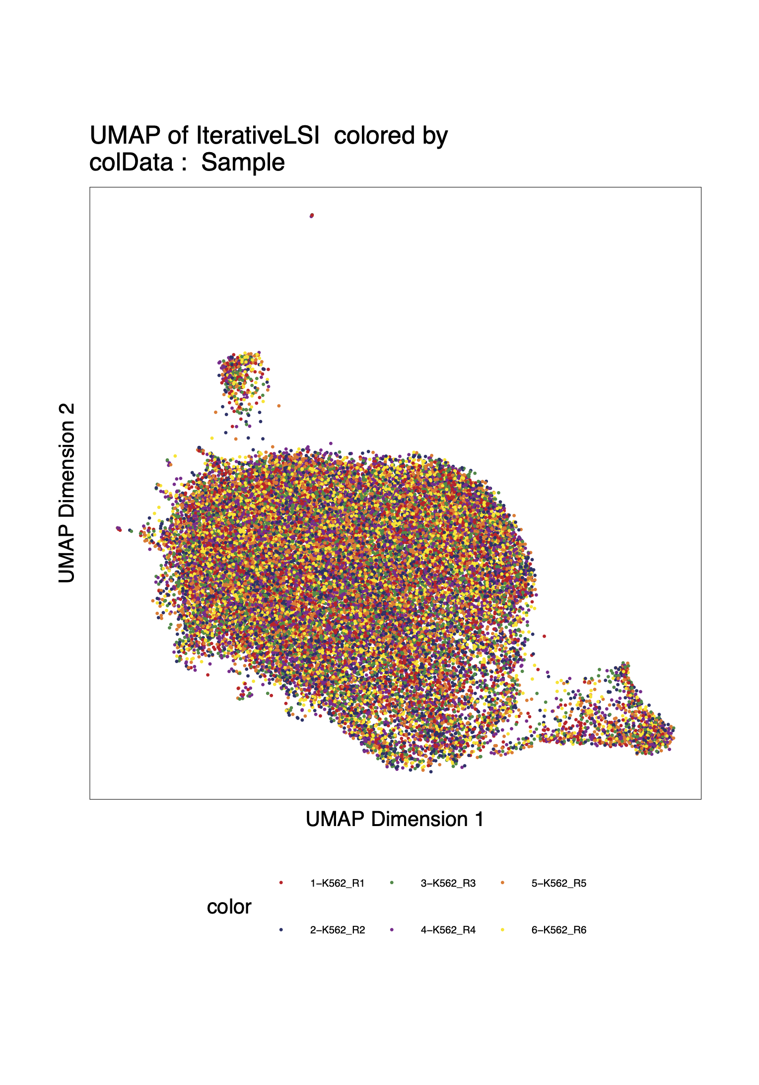
#Plot UMAP Embeddings
p1 <- plotEmbedding(proj, colorBy = "cellColData", name = "Sample", pal=pal4,labelMeans = FALSE)
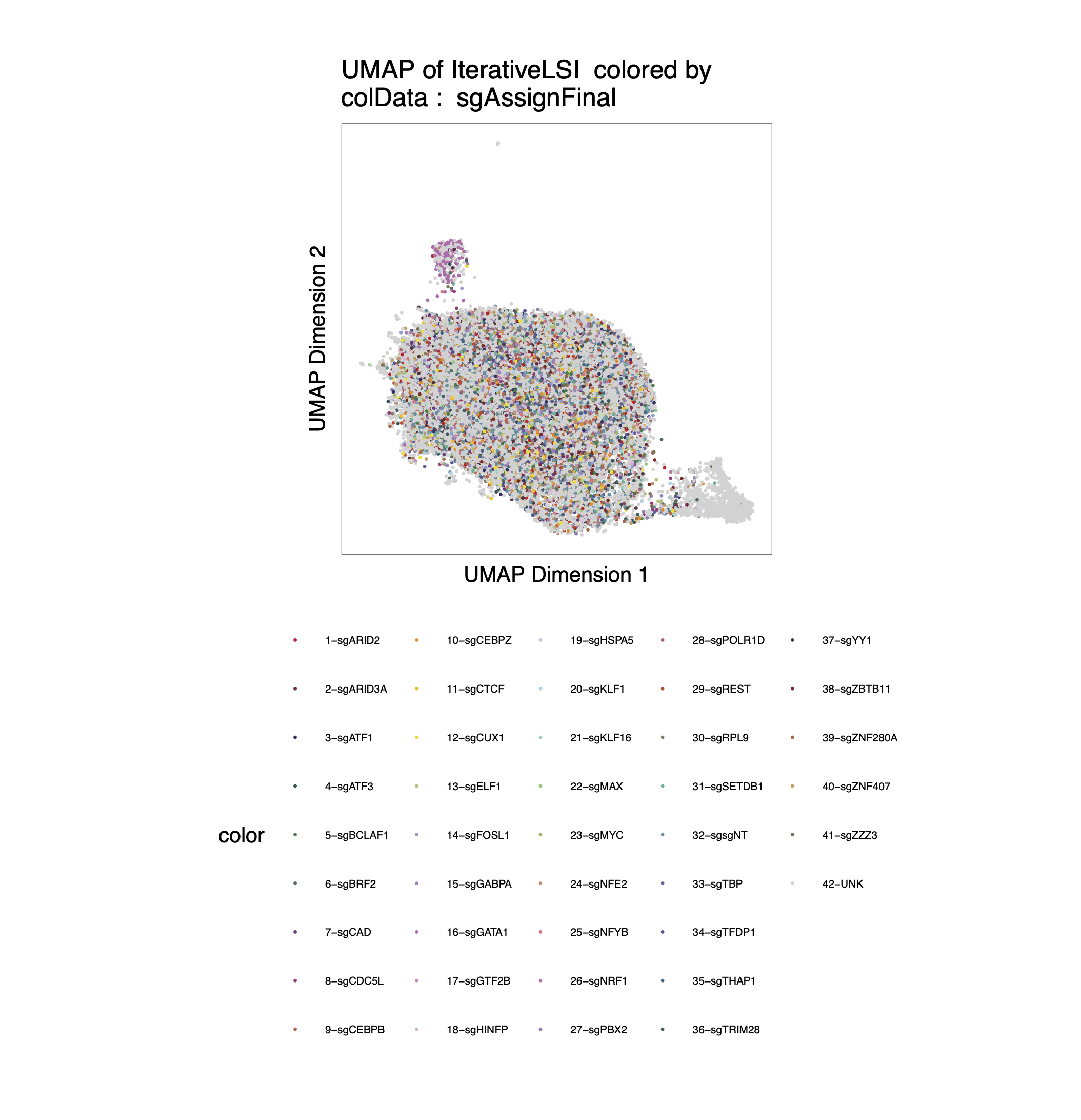
p2 <- plotEmbedding(proj, colorBy = "cellColData", name = "sgAssignFinal", pal = pal3, labelMeans = FALSE)
ggsave(
"./Plots/K562_UMAP_p1.pdf", p1,
scale = 1,
width = 8,
height = 8,
dpi = 600)
ggsave(
"./Plots/K562_UMAP_p2.pdf", p2,
scale = 1,
width = 8,
height = 8,
dpi = 600)
#Call Peaks using sgAssignments
proj <- addGroupCoverages(proj, groupBy = "sgAssignFinal")
saveRDS(proj, "Save-ArchRProject-W-sgRNA-Assignments-2.rds")
proj <- addReproduciblePeakSet(proj,
groupBy = "sgAssignFinal",
pathToMacs2 = "/Users/zeyulu/anaconda3/bin/macs2")
proj <- addPeakMatrix(proj)
#Filter These sgRNA non-targetting because they seem to exhibit some differences from the other sgNT
#This step helps a bit, but is not necessary to get differential results
bgd <- grep("sgNT", proj$sgIndividual, value=TRUE) %>% unique
bgd
bgd <- bgd[!grepl("-11|-12|-8|-5|-6", bgd)]
proj$sgAssignClean <- proj$sgAssignFinal
proj$sgAssignClean[grepl("-11|-12|-8|-5|-6", proj$sgIndividual)] <- "UNK"
#Sort sgRNA Targets so Results are in alphabetical order
useGroups <- sort(unique(proj$sgAssignClean)[unique(proj$sgAssignClean) %ni% c("UNK")])
bgdGroups <- unique(grep("sgNT", proj$sgAssignClean,value=TRUE))
useGroups
bgdGroups
proj
#Differential Peaks
diffPeaks <- getMarkerFeatures(
ArchRProj = proj,
testMethod = "binomial",
binarize = TRUE,
useMatrix = "PeakMatrix",
useGroups = useGroups,
bgdGroups = bgdGroups,
groupBy = "sgAssignClean",
bufferRatio = 0.95,
maxCells = 250,
threads = 10
)
dir.create("./K562/MarkerSet/", showWarnings = FALSE, recursive = TRUE)
markerLists<-getMarkers(DiffPeaks,cutOff = "FDR <= 0.05 & abs(Log2FC) >= 2")
unique_TF_names<-names(markerLists)
unique_TF_names
for(i in 1:length(markerLists)){
if(nrow(markerLists[[i]])>0){
gr<-GRanges(
seqnames = as.character(markerLists[[unique_TF_names[i]]]$seqnames),
ranges = IRanges(start = markerLists[[unique_TF_names[i]]]$start, end = markerLists[[unique_TF_names[i]]]$end),
strand = "*",
score = abs(markerLists[[unique_TF_names[i]]]$Log2FC))
export.bed(gr,paste0("./K562/MarkerSet/",unique_TF_names[i],".bed"))
}
}
We can generate the UMAP plots colored by sample replicates or sgRNA target.
By sample replicate:
By sgRNA target:
After processing, we obtain *.bed files for each sgRNA target.

Next we apply BIT to all datasets to generate the ranks:
Noticed in plot 1 and in the original publication, the sgGATA1 targeted cells are more significantly differ from the rest cells. We show the top10 TRs ranked by BIT in the sgGATA1 targeted cells:
data_read<-read.csv(paste0("./K562/bit/sgGATA1_rank_table.csv"))
data<-data.frame(Group="sgGATA1 targeted cells",
                 Label=data_read[1:20,"TR"],
                 Value=data_read[1:20,"BIT_score"],
                 Upper=data_read[1:20,"BIT_score_upper"],
                 Lower=data_read[1:20,"BIT_score_lower"])
data$Label<-factor(data$Label,levels=rev(data$Label))
top10_data <- data[1:10, ]

p1<-ggplot(top10_data, aes(x = Label, y = Value)) +
  geom_col(fill="#BADDF5",colour="black",size=0.25) +
  geom_errorbar(aes(ymin = Lower, ymax = Upper), width = 0.5, color = "black", size = 0.35) +
  coord_flip() +  # Flip coordinates to make the bar plot horizontal
  facet_grid(.~Group, scales = "free_y") +  # Facet by group, allowing free scales on the y-axis
  labs(title = "",
       x = "Top 10 Identified TRs",
       y = "") + scale_y_continuous(limits=c(0,0.05),breaks=seq(0,0.5,by=0.01),expand = c(0,0)) +
  theme_bw() +  # Using a minimal theme
  theme(axis.text.x = element_text(color="black",size=12),
        axis.text.y = element_text(color="black",size=12),axis.title.y=element_text(size=14),
        legend.position = "none", plot.margin = unit(c(0,0.5,0,0),"cm")) +theme(strip.background = element_rect(fill="#DBD1B6"),
                                                                                strip.text = element_text(size=12, colour="black"))
p1
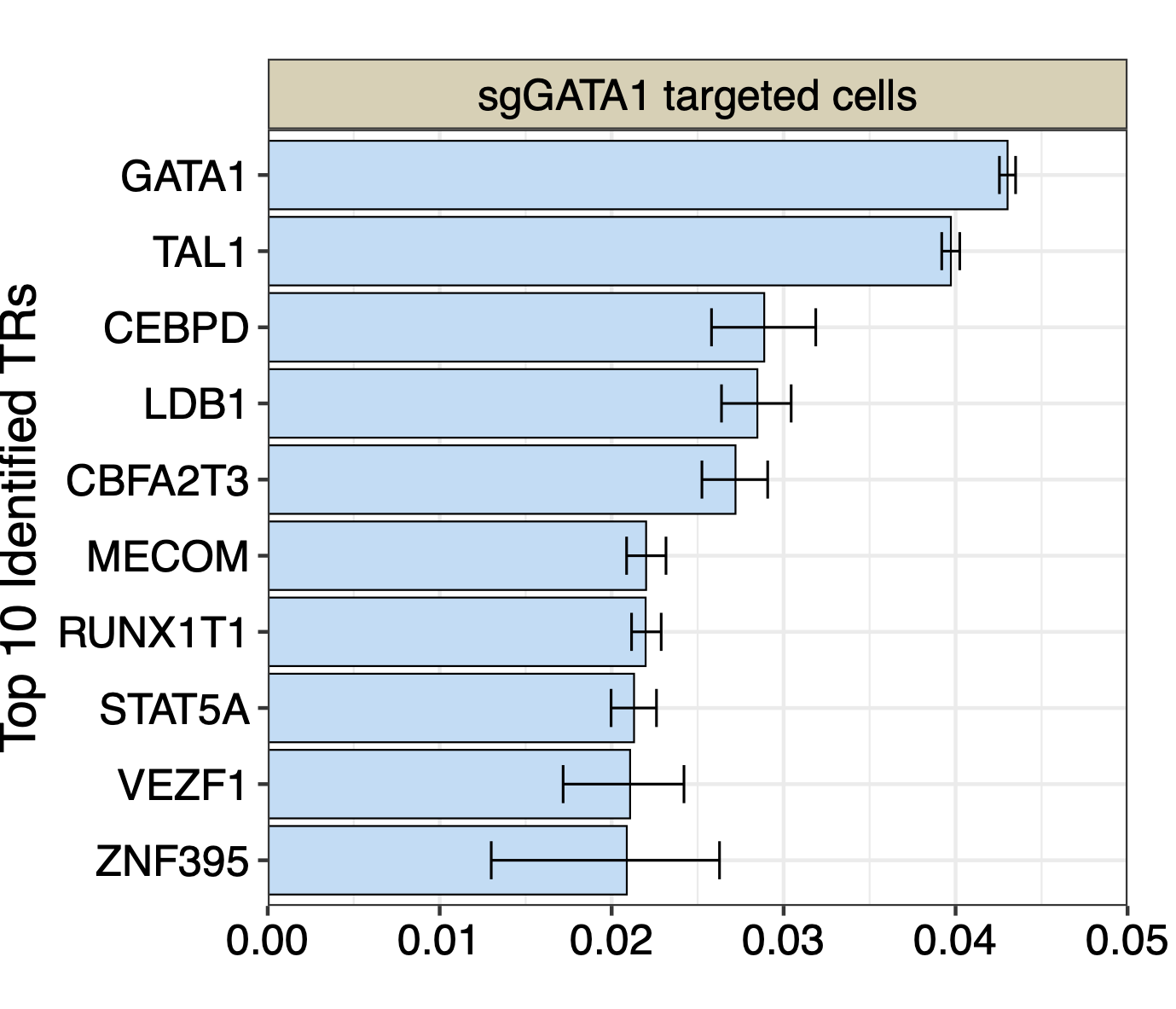
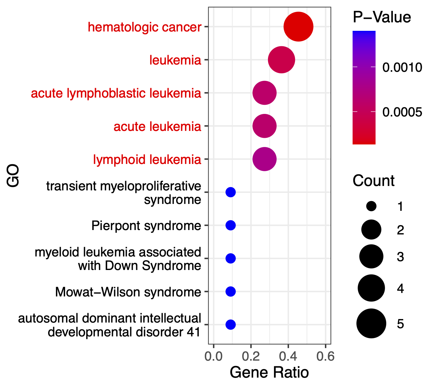
We can see BIT successfully rank GATA1 to top 1. We next conduct GO enrichment analysis using top 20 TRs identified by BIT in sgGATA1-targeted cells:
The GO enrichment analysis result plot is:
Next, we apply state-of-the-art methods to analyze the generated *.bed files and extract outputs from each method. The following tools are used:
We merged the outputs from each sgRNA-targeted-cells cluster to get the merged output table for each method.
library(stringr)
library(gridExtra)
library(dplyr)
library(tidyr)

work_dir<-"/Users/zeyulu/Desktop/Project/BIT/revision_data/K562/"

bart2_table<-read.csv(paste0(work_dir,"bart2_table.csv"))
chip_atlas_table<-read.csv(paste0(work_dir,"chip_atlas_table.csv"))
bit_table<-read.csv(paste0(work_dir,"bit_table.csv"))
icistarget_table<-read.csv(paste0(work_dir,"icistarget_table.csv"))
whichtf_files<-read.csv(paste0(work_dir,"whichtf_table.csv"))
homer_table<-read.csv(paste0(work_dir,"homer_table.csv"))

###############################################################

table_lists<-list("BIT"=bit_table,
                  "BART2"=bart2_table,
                  "ChIP-Atlas"=chip_atlas_table,
                  "HOMER"=homer_table,
                  "i-cisTarget"=icistarget_table,
                  "WhichTF"=whichtf_table)
After summarizing all tables, we proceed to generate the plots.
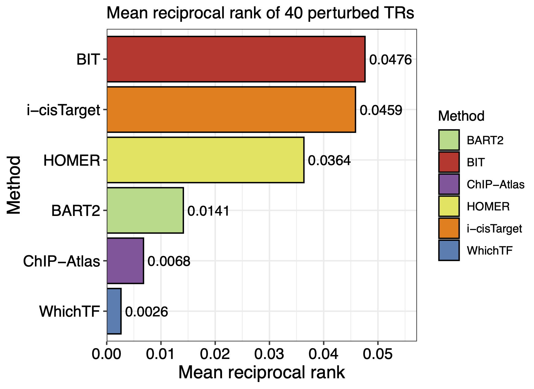
First, we calculate the Mean Reciprocal Rank (MRR) for the 40 perturbed TRs across different methods. Simultaneously, we count the number of TRs ranked within the top 10 and top 50 by each method.
##############
MRR_cal<-function(rank_res){
  rank_res<-1/rank_res
  rank_res[is.na(rank_res)]=0
  return(mean(rank_res))
}

Method_names<-names(table_lists)

MRR_res<-c()
Top50<-c()
Top10<-c()

for(i in 1:6){
  df=table_lists[[Method_names[i]]]
  rank_res<-c()
  Method_name<-Method_names[i]
  for(i in 1:ncol(df)){
    if(length(which(df[,i]==colnames(df)[i]))>0){
      rank_res<-c(rank_res,which(df[,i]==colnames(df)[i]))
    }else{
      rank_res<-c(rank_res,NA)
    }
  }
  Top10<-c(sum(rank_res<=10,na.rm=TRUE),Top10)
  Top50<-c(sum(rank_res<=50,na.rm=TRUE),Top50)
  MRR_res<-c(MRR_cal(rank_res),MRR_res)
}
names(MRR_res)<-rev(Method_names)
names(Top10)<-rev(Method_names)
names(Top50)<-rev(Method_names)

#> MRR_res
#    WhichTF i-cisTarget       HOMER  ChIP-Atlas       BART2         BIT
#0.002632788 0.045862471 0.036355700 0.006783940 0.014126888 0.047616672
#> Top10
#    WhichTF i-cisTarget       HOMER  ChIP-Atlas       BART2         BIT
#          0           3           2           1           1           3
#> Top50
#    WhichTF i-cisTarget       HOMER  ChIP-Atlas       BART2         BIT
#          1           5           4           2           4           9
Next, we visualize the MRRs for the six methods using the following plot:
MRR_df
Top_df
MRR_df<-data.frame(MRR_res)
Top_df<-data.frame(Top10)
Top_df$Top50<-Top50
MRR_df$Method<-rownames(MRR_df)
Top_df$Method<-rownames(Top_df)

ggplot(MRR_df, aes(x = reorder(Method, MRR_res), y = MRR_res, fill = Method)) +
  geom_bar(stat = "identity", color = "black", linewidth = 0.5) +  # Add border to bars
  geom_text(aes(label = round(MRR_res, 4)), hjust = -0.1, size = 4) +  # Add text labels
  coord_flip() +  # Flip coordinates for horizontal bars
  labs(x = "Method", y = "Mean reciprocal rank", title = "Mean reciprocal rank of 40 perturbed TRs") +
  theme_bw() + theme(axis.title.x = element_text(size=14,color="black"),
                     axis.title.y = element_text(size=14,color="black"),
                     axis.text.x = element_text(size=12,color="black"),
                     axis.text.y = element_text(size=12,color="black"))+
scale_fill_manual(values = c("BIT" = "#D2352C", "BART2" = "#ADDB88", "HOMER" = "#E3E457", "ChIP-Atlas" = "#8E549E","i-cisTarget"="#FA8002","WhichTF"="#497EB2")) +  # Custom colors
  scale_y_continuous(limits=c(0,0.052),expand = expansion(mult = c(0, 0.1)))  # Adjust y-axis to fit text labels
Figure:
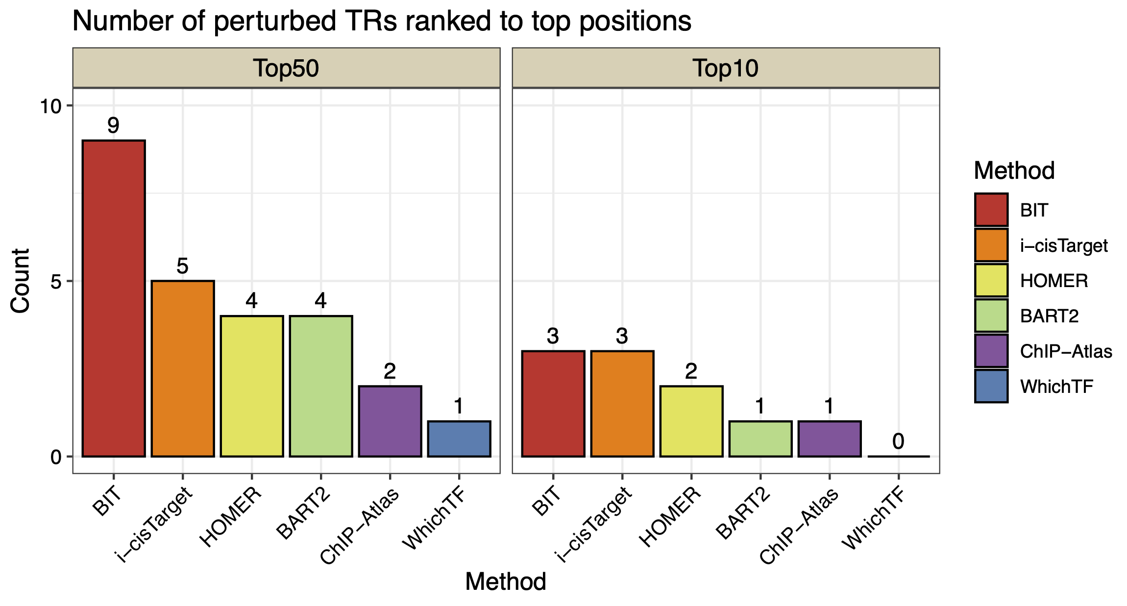
We also visualize the number of TRs ranked within the top 10 and top 50 by each method:
Top_df_long <- Top_df %>%
  pivot_longer(cols = starts_with("Top"), names_to = "Group", values_to = "Value")

Top_df_long$Method<-factor(Top_df_long$Method,levels=c("BIT","i-cisTarget","HOMER","BART2","ChIP-Atlas","WhichTF"))
Top_df_long$Group<-factor(Top_df_long$Group,levels=c("Top50","Top10"))

ggplot(Top_df_long, aes(x = Method, y = Value, fill = Method)) +
geom_bar(stat = "identity", position = position_dodge(),color="black") +
facet_wrap(~ Group, ncol = 2) +  # Separate into two groups (Top10 and Top50)
labs(title = "Number of perturbed TRs ranked to top positions",
     x = "Method",
     y = "Count",
     fill = "Method") + geom_text(aes(label = Value), hjust = 0.5,vjust=-0.5, size = 4) +
theme_bw() + scale_y_continuous(breaks = c(0,10,5),limits=c(0,10))+ scale_fill_manual(values = c("BIT" = "#D2352C", "BART2" = "#ADDB88", "HOMER" = "#E3E457", "ChIP-Atlas" = "#8E549E","i-cisTarget"= "#FA8002","WhichTF"="#497EB2")) +  # Custom colors
theme(axis.text.x = element_text(size=10,angle = 45, hjust = 1,color="black"), axis.title.y = element_text(size=12,color="black"),
      axis.title.x = element_text(size=12,color="black"),
      axis.text.y = element_text(size=10,color="black"), title=element_text(size=12,color="black"),strip.background = element_rect(fill="#DBD1B6"),
      strip.text = element_text(size=12, colour="black"))  # Rotate x-axis labels for better readability
Figure: