10xGenomics PBMCs cell-type-specific TRs

We utilize SnapATAC2 to process single-cell ATAC-seq (scATAC-seq) data obtained from 10xGENOMICS. . The detailed usage guide for SnapATAC2 can be found in the SnapATAC2-manual. We used SnapATAC2 v2.6.0 for our analysis.

For improved efficiency, some steps require a GPU to accelerate model training.

# -----------------------------
# Import Required Libraries
# -----------------------------
import warnings
warnings.filterwarnings("ignore")  # Ignore warning messages for cleaner output

import snapatac2 as snap         # Library for scATAC-seq analysis
import anndata as ad             # Handling annotated data matrices
import pandas as pd              # Data manipulation and analysis
import scanpy as sc              # Single-cell analysis package
import scvi                     # Probabilistic modeling for single-cell omics data
import os                       # For directory operations
import matplotlib.pyplot as plt # For plotting

# -----------------------------
# Set Global Settings & Seed
# -----------------------------
scvi.settings.seed = 2          # Set random seed for reproducibility
print("i")                     # Print a simple indicator (optional)

# -----------------------------
# Data Loading and Preprocessing
# -----------------------------
# Load a reference dataset from the provided multiome dataset
reference = snap.read(snap.datasets.pbmc10k_multiome(), backed=None)

# Load an ATAC dataset from a local file
atac = snap.read("./10XGENOMICS/pbmc.h5ad", backed=None)

# Generate a gene expression matrix from the ATAC dataset using gene annotations for hg38
query = snap.pp.make_gene_matrix(atac, gene_anno=snap.genome.hg38)

# Initialize the cell type annotation for the query dataset as missing values
query.obs['cell_type'] = pd.NA

# Concatenate the reference and query datasets into one AnnData object
data = ad.concat(
    [reference, query],
    join='inner',                # Keep only features present in both datasets
    label='batch',               # Create a batch label to differentiate datasets
    keys=["reference", "query"],
    index_unique='_'
)

# -----------------------------
# Filter and Identify Highly Variable Genes
# -----------------------------
sc.pp.filter_genes(data, min_cells=5)  # Keep genes expressed in at least 5 cells

# Identify and subset to the top 5000 highly variable genes using Seurat v3 method
sc.pp.highly_variable_genes(
    data,
    n_top_genes=5000,
    flavor="seurat_v3",
    batch_key="batch",  # Consider batch effects when identifying variable genes
    subset=True
)

# -----------------------------
# Setup and Train SCVI Model
# -----------------------------
# Configure the AnnData object for SCVI with batch key
scvi.model.SCVI.setup_anndata(data, batch_key="batch")

# Initialize the SCVI model with 2 layers and 30 latent dimensions
vae = scvi.model.SCVI(
    data,
    n_layers=2,
    n_latent=30,
    gene_likelihood="nb",     # Negative binomial likelihood for gene expression
    dispersion="gene-batch"   # Model dispersion per gene and batch
)

# Train the SCVI model (using early stopping to prevent overfitting)
vae.train(max_epochs=2000, early_stopping=True)

# -----------------------------
# Prepare Data for SCANVI
# -----------------------------
# Initialize a new column for cell type labels with a default value 'Unknown'
data.obs["celltype_scanvi"] = 'Unknown'

# Identify the reference cells (where batch is "reference")
ref_idx = data.obs['batch'] == "reference"
# For reference cells, assign the known cell type labels
data.obs["celltype_scanvi"][ref_idx] = data.obs['cell_type'][ref_idx]

# Initialize the SCANVI model using the pretrained SCVI model and provided labels
lvae = scvi.model.SCANVI.from_scvi_model(
    vae,
    adata=data,
    labels_key="celltype_scanvi",
    unlabeled_category="Unknown"
)

# Train the SCANVI model further with a maximum of 2000 epochs and sample 100 cells per label
lvae.train(max_epochs=2000, n_samples_per_label=100)

# -----------------------------
# Obtain Predictions and Latent Representation
# -----------------------------
# Predict cell type labels using SCANVI and store the predictions in a new column
data.obs["C_scANVI"] = lvae.predict(data)
# Get the latent representation from SCANVI for downstream analysis and visualization
data.obsm["X_scANVI"] = lvae.get_latent_representation(data)

# -----------------------------
# Compute UMAP Embedding
# -----------------------------
# Compute the nearest neighbors using the SCANVI latent representation
sc.pp.neighbors(data, use_rep="X_scANVI")
# Calculate UMAP coordinates for visualization
sc.tl.umap(data)

# Save the processed AnnData object with UMAP embedding to disk (compressed)
data.write("./10XGENOMICSpbmc10k.h5ad", compression="gzip")

# -----------------------------
# Annotate ATAC Data with Predicted Cell Types
# -----------------------------
# Map predicted cell type labels from the integrated data to the original ATAC dataset
atac.obs['Cell_Types'] = data.obs.loc[atac.obs_names + '_query']['C_scANVI'].to_numpy()

# Save the ATAC data with annotations
atac.write("./10XGENOMICS/pbmc10k_annotated.h5ad", compression="gzip")

# -----------------------------
# Peak Calling and Matrix Generation
# -----------------------------
# Run MACS3 peak calling on the data grouped by merged cell types
snap.tl.macs3(data, groupby='Cell_Types')
# Merge peaks across groups using hg38 annotations
peaks = snap.tl.merge_peaks(data.uns['macs3'], snap.genome.hg38)
# Create a peak accessibility matrix using the merged peaks
peak_mat = snap.pp.make_peak_matrix(data, use_rep=peaks['Peaks'])

# Create a new directory to save CSV outputs, using the current seed in the folder name
os.mkdir("./10XGENOMICS/csv/scATAC_Peaks_" + str(scvi.settings.seed))

# -----------------------------
# Set Plotting Parameters for High Resolution
# -----------------------------
plt.rcParams['figure.dpi'] = 1000    # High resolution for displaying figures
plt.rcParams['savefig.dpi'] = 1000   # High resolution for saving figures
plt.rcParams['figure.figsize'] = [8, 8]  # Set default figure size

# -----------------------------
# UMAP Plotting of Cell Types
# -----------------------------
# Compute UMAP embedding with a fixed random state for reproducibility
snap.tl.umap(data, random_state=15)

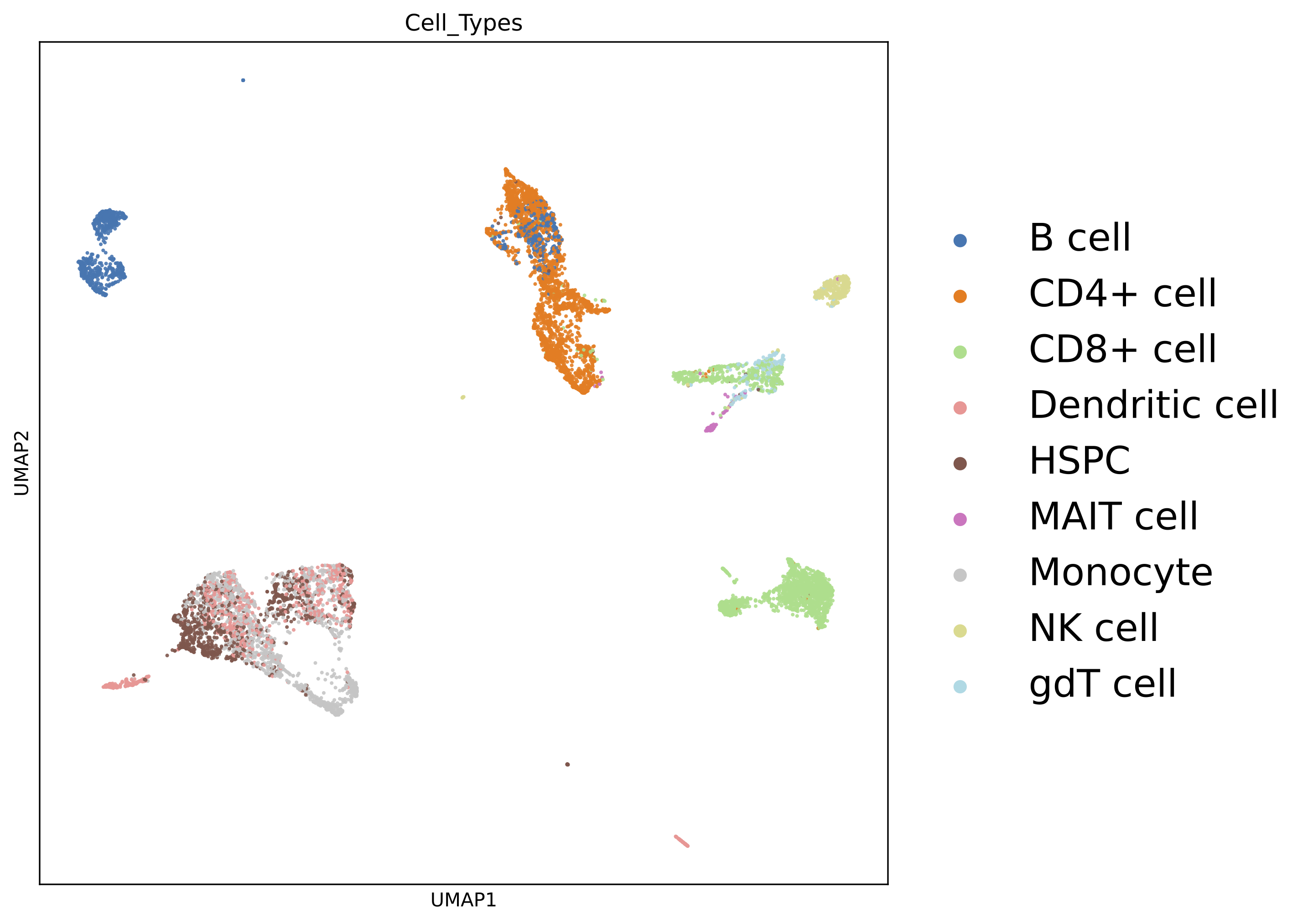
# Plot the UMAP embedding colored by cell types with custom styling
sc.pl.umap(
    data,
    color="Cell_Types",
    size=15,                # Increase point size for visibility
    alpha=0.9,              # Slight transparency to visualize density
    legend_fontsize=20,
    legend_fontweight='bold',
    frameon=True,           # Display the frame for clarity
    ncols=2,                # Organize legend into two columns
    show=False,
    save='umap_plot_Test.pdf'
)

# -----------------------------
# Process and Save Gene Expression Matrix
# -----------------------------
# Create a gene expression matrix using hg38 annotations
gene_matrix = snap.pp.make_gene_matrix(data, snap.genome.hg38)
print(gene_matrix)

# Filter genes expressed in fewer than 5 cells
sc.pp.filter_genes(gene_matrix, min_cells=5)
# Normalize total counts per cell
sc.pp.normalize_total(gene_matrix)
# Log-transform the normalized counts
sc.pp.log1p(gene_matrix)

# Apply MAGIC imputation (approximate solver) to smooth gene expression data
sc.external.pp.magic(gene_matrix, solver="approximate")
# Transfer UMAP coordinates from 'data' to gene_matrix for consistent visualization
gene_matrix.obsm["X_umap"] = data.obsm["X_umap"]

# Save the processed gene matrix to disk (compressed)
gene_matrix.write("pbmc10k_gene_mat.h5ad", compression='gzip')

# Set global figure parameters for scanpy plots
sc.set_figure_params(scanpy=True, dpi=1000, dpi_save=1000, fontsize=24, figsize=[10, 10])

# -----------------------------
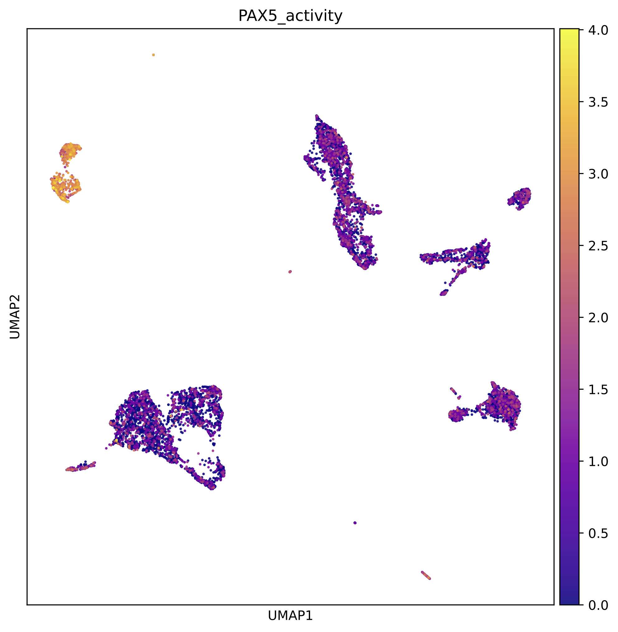
# Plot Marker Genes on UMAP
# -----------------------------
marker_genes = []  # Define marker genes to visualize on UMAP (fill in with gene names)

# Reload the gene matrix to ensure data consistency
gene_matrix = snap.read("pbmc10k_gene_mat.h5ad", backed=None)

# Loop through each marker gene and plot its expression on the UMAP
for i in range(len(marker_genes)):
    sc.pl.umap(
        gene_matrix,
        use_raw=False,
        color=marker_genes[i],
        size=15,                # Increase point size for better visibility
        alpha=0.9,              # Slight transparency to indicate density
        frameon=True,           # Show a frame around the plot
        ncols=5,                # Organize legends into 5 columns if needed
        show=False,
        save='umap_plot_Test_UMAP_PBMCs_' + marker_genes[i] + '.pdf',
        color_map="plasma"      # Use the 'plasma' color map for gene expression
    )

The previous pipeline can generate the below UMAP plots:

Colored by cell types:

Colored by PAX5 gene activity:

We also get the marker peaks of each cell type:

marker_peaks=snap.tl.marker_regions(peak_mat, groupby='Cell_Types', pvalue=0.01)
for keys in marker_peaks.keys():
        elements=marker_peaks[keys]
        chromosomes = []
        starts = []
        ends = []
        for element in elements:
            # Split each element into chromosome, start, and end
            chromosome, positions = element.split(':')
            start, end = positions.split('-')
            # Append the results to the corresponding lists
            chromosomes.append(chromosome)
            starts.append(start)
            ends.append(end)
        df = pd.DataFrame({'Chrom': chromosomes,'Start': starts,'End': ends})
        df.to_csv("./10XGENOMICS/csv/scATAC_Peaks_"+scvi.settings.seed+"/"+keys.replace(" ","_")+".csv",index=False)
    print("./10XGENOMICS/csv/scATAC_Peaks_"+scvi.settings.seed+" Done")

cell-type-specific marker regions:

We run BIT on each of the region set:

work_dir<-"./10XGENOMICS/csv/"
work_files<-list.files(work_dir)
output_path<-"./10XGENOMICS/bit/"
dir.create(output_path, showWarnings = FALSE, recursive = TRUE)
for(i in seq_along(work_files)){
  BIT(paste0(work_dir,work_files[i]), output_path=output_dir, format="csv", bin_width=1000, genome="hg38")
}

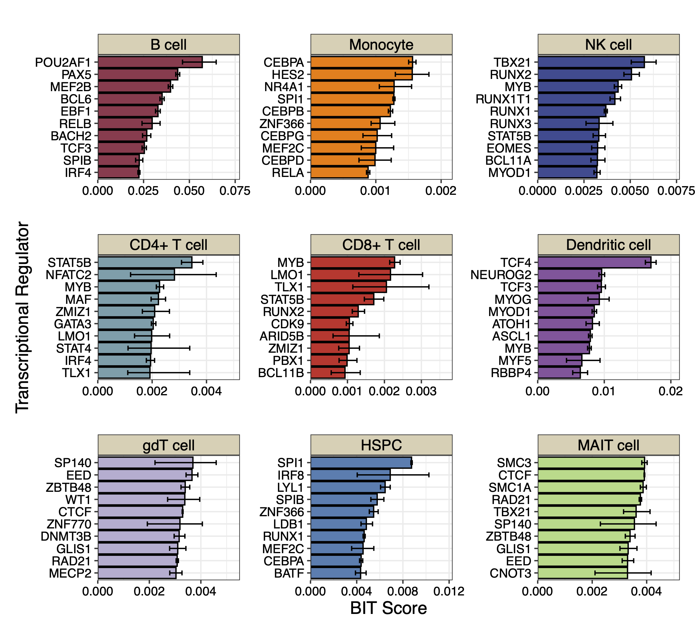
We plot the top 10 TRs identified by BIT in each cell type along with the 95% credible intervals:

library(patchwork)
work_dir<-"./10XGENOMICS/bit/"
work_files_BIT<-list.files(work_dir,pattern="*_rank_table.csv")
work_files_BIT<-work_files_BIT[c(1,8,9,2,3,4,5,6,7)]

cell_names<-sapply(strsplit(work_files_BIT,"_rank",fixed=TRUE),function(x){return(x[[1]])})
cell_names<-tools::toTitleCase(cell_names)
cell_names<-c("B cell","Monocyte","NK cell","CD4+ T cell","CD8+ T cell","Dendritic cell","gdT cell","HSPC","MAIT cell")
colors<-c("#9B3A4D","#FC8002","#394A92","#70A0AC","#D2352C","#8E549E","#BAAFD1","#497EB2","#ADDB88")
plot_list<-list()
for(i in 1:9){
  table<-read.csv(paste0(work_dir,work_files_BIT[i]),row.names=1)
  data<-data.frame(TR=table$TR[1:10],
                   Score=table$BIT_score[1:10],
                   Lower=table$BIT_score_lower[1:10],
                   Upper=table$BIT_score_upper[1:10],
                   group=cell_names[i])
  data$TR<-factor(data$TR,levels=rev(data$TR))
  plot_list[[i]]<-ggplot(data, aes(x = TR, y = Score)) +
    geom_bar(stat = "identity", fill = colors[i], color = "black") +
    geom_errorbar(aes(ymin = Lower, ymax = Upper), width = 0.4) +
    coord_flip() +
    theme_bw() + scale_y_continuous(limits = c(0, max(data$Upper)*1.2),breaks = scales::breaks_extended(n = 4),expand = c(0,0)) + facet_grid(.~group)+
    labs(
      title = "",
      x = "Transcriptional Regulator",
      y = "BIT Score"
    )+theme(title=element_text(size=9),plot.margin=unit(c(0.25,0.25,0.25,0.25),"cm"),axis.text.y = element_text(size=10,color="black"),
            axis.text.x = element_text(size=10,color="black"),
            axis.title.x = element_text(size=14,color="black"),
            axis.title.y = element_text(size=14,color="black"),
            strip.background = element_rect(fill="#DBD1B6"),
            strip.text = element_text(size=12, colour="black",margin=ggplot2::margin(1,1,1,1,"mm")))
}

p_combined<-plot_list[[1]]+plot_list[[2]]+ plot_list[[3]] +
  plot_list[[4]]+plot_list[[5]]+plot_list[[6]] +
  plot_list[[7]]+plot_list[[8]]+plot_list[[9]]+ plot_layout(ncol=3,guides="collect",axis_titles = "collect")
print(p_combined)

We can also plot the GO enrichment analysis results of each cell type:

split_go_term <- function(term) {
  words <- strsplit(term, " ")[[1]]
  n_words <- length(words)

  # Find split points for 2-3 lines
  if(n_words <= 3) {
    split_at <- ceiling(n_words/2)
  } else {
    split_at <- c(ceiling(n_words/3), ceiling(n_words*2/3))
  }

  # Split words into groups
  groups <- split(words, cut(seq_along(words), breaks = c(0, split_at, n_words)))

  # Combine with newlines
  paste(sapply(groups, paste, collapse = " "), collapse = "\n")
}

integer_breaks <- function(x, n = 4) {
  x <- x[!is.na(x)]
  if (length(x) == 0) return(numeric())
  rng <- range(x)
  breaks <- floor(rng[1]):ceiling(rng[2])
  breaks <- unique(round(breaks))
  if (length(breaks) > n) {
    breaks <- breaks[seq(1, length(breaks), length.out = n)]
  }
  breaks
}

work_files_BIT
plot_list<-list()

for(i in 1:9){
  table<-read.csv(paste0(work_dir,work_files_BIT[i]),row.names=1)
  data<-data.frame(TR=table$TR[1:20],
                   group=cell_names[i])
  BIT_gene_ids<-bitr(data$TR,fromType = "SYMBOL",toType = "ENTREZID",OrgDb="org.Hs.eg.db")
  BIT_Results=enrichGO(gene          = BIT_gene_ids$ENTREZID[1:20],
                       OrgDb = "org.Hs.eg.db",
                       ont = "BP",
                       pAdjustMethod = "BH",
                       pvalueCutoff  = 0.01,
                       qvalueCutoff  = 0.05)
  GO_BIT_table<-head(BIT_Results,5)
  GO_PLOT_Table_BIT<-data.frame(GO=GO_BIT_table$Description,
                                GeneRatio=Trans_to_double(GO_BIT_table),
                                Pvalue=GO_BIT_table$pvalue,
                                Count=GO_BIT_table$Count)
  GO_PLOT_Table_BIT$GO <- sapply(GO_PLOT_Table_BIT$GO, split_go_term)
  plot_list[[i]] <- ggplot(GO_PLOT_Table_BIT, aes(x = GeneRatio, y = reorder(GO, -Pvalue), size = Count, color = Pvalue)) +
    geom_point() +
    # Fix Pvalue color legend (4 breaks, no overlap)
    scale_color_gradient(
      low = "red",
      high = "blue",
      limits = c(min(GO_BIT_table$pvalue), max(GO_BIT_table$pvalue)),
      breaks = scales::breaks_pretty(n = 4), # 4 breaks # 2 decimal places
      guide = guide_colorbar(
        order = 1,
        title.position = "top",
        barheight = unit(1.6, "cm"),
        ticks = FALSE
      )
    ) +
    # Fix Count size legend (integer breaks)
    scale_size_continuous(
      breaks = integer_breaks(GO_PLOT_Table_BIT$Count, n = 4), # 4 integer breaks
      range = c(2, 5), # Adjust point sizes
      guide = guide_legend(
        order = 2,
        title.position = "top",
        override.aes = list(color = "black")
      )
    ) +
    theme_bw() +
    labs(y = "GO", x = "Gene Ratio", color = "P-Value", size = "Count") +
    theme(
      text = element_text(size = 12),
      legend.position = "right",
      legend.box = "vertical",
      legend.spacing.y = unit(0.1, "cm"),
      legend.margin = margin(0, 0, 0, 0),
      axis.text.y = element_text(color = "black")
    ) +
    xlim(c(0.0, 0.6))
}
p_combined<-plot_list[[1]]+plot_list[[2]]+ plot_list[[3]] +
plot_list[[4]]+plot_list[[5]]+plot_list[[6]] +
  plot_list[[7]]+plot_list[[8]]+plot_list[[9]]+ plot_layout(ncol=3,axis_titles = "collect")

print(p_combined)

We use SnapATAC2’s built-in motif enrichment analysis method to derive the corresponding motif enrichment results:

os.makedirs('./10XGENOMICS/motifs/', exist_ok=True)
motifs = snap.tl.motif_enrichment(
    motifs=snap.datasets.cis_bp(unique=True),
    regions=marker_peaks,
    genome_fasta=snap.genome.hg38,
)
for keys in motifs.keys():
                elements=motifs[keys]
                df=elements.to_pandas()
                df=df.sort_values(by="adjusted p-value",ascending=True)
                df.to_csv('./10XGENOMICS/motifs/pbmc10k_'+str(i)+"/"+keys+'_motifs.csv',index=False)

To generate results using ArchR and scBasset, you cannot use the marker peaks produced by SnapATAC2. Instead, you need to process the scATAC-seq data directly from the fragments. We recommend consulting the original manuals for further details: (1) ArchR manual (2) scBasset manual.

For ArchR:

# -----------------------------------------------
# Configuration & Library Setup
# -----------------------------------------------

library(ArchR)              # Load the ArchR package for scATAC-seq analysis
set.seed(42)                # Set seed for reproducibility
addArchRGenome("hg38")      # Add human genome reference (hg38)

# -----------------------------------------------
# Define Input Files
# -----------------------------------------------
# Specify input file(s) with sample names and paths.
inputFiles <- c("PBMCs10k" = "./10XGENOMICS/PBMCs/pbmc10k.tsv.gz")

# -----------------------------------------------
# Create Arrow Files
# -----------------------------------------------
# Arrow files are a specialized file format used by ArchR to store data.
ArrowFiles <- createArrowFiles(
  inputFiles = inputFiles,         # Input file(s)
  sampleNames = names(inputFiles), # Use the names from the inputFiles vector
  filterTSS = 4,                   # Minimum TSS enrichment score; avoid setting too high initially
  filterFrags = 1000,              # Minimum number of fragments per cell
  addTileMat = TRUE,               # Create a tile matrix for downstream analysis
  addGeneScoreMat = TRUE           # Generate a gene score matrix
)

# -----------------------------------------------
# Calculate Doublet Scores
# -----------------------------------------------
# Identify potential doublets (artificially merged cells) in the dataset.
doubScores <- addDoubletScores(
  input = ArrowFiles,              # Use the previously created Arrow files
  k = 10,                          # Number of neighbors considered for "pseudo-doublet" estimation
  knnMethod = "UMAP",              # Use UMAP embedding for nearest neighbor search
  LSIMethod = 1                    # Specify LSI method (typically 1)
)

# -----------------------------------------------
# Create ArchR Project
# -----------------------------------------------
# The ArchR project organizes data and metadata for further analysis.
proj <- ArchRProject(
  ArrowFiles = ArrowFiles,                                         # Input Arrow files
  outputDirectory = "/projects/dheitjan/BIT/zeyul/BIT/ArchR/PBMC",  # Directory to store project outputs
  copyArrows = TRUE                                                 # Maintain an unaltered copy of the Arrow files
)

# -----------------------------------------------
# Filter Out Doublets
# -----------------------------------------------
proj <- filterDoublets(ArchRProj = proj)  # Remove cells flagged as doublets

# -----------------------------------------------
# Dimensionality Reduction and Clustering
# -----------------------------------------------
# 1. Perform iterative Latent Semantic Indexing (LSI) for dimensionality reduction
proj <- addIterativeLSI(ArchRProj = proj, useMatrix = "TileMatrix", name = "IterativeLSI")

# 2. Cluster cells using the reduced dimensions from IterativeLSI
proj <- addClusters(input = proj, reducedDims = "IterativeLSI")

# 3. Generate a UMAP embedding for visualization
proj <- addUMAP(ArchRProj = proj, reducedDims = "IterativeLSI")
p2 <- plotEmbedding(
  ArchRProj = proj,
  colorBy = "cellColData",  # Color cells by metadata (e.g., clusters)
  name = "Clusters",
  embedding = "UMAP"
)

# -----------------------------------------------
# Data Imputation and Saving Project
# -----------------------------------------------
proj <- addImputeWeights(proj)                # Impute missing values to smooth data visualization
proj <- saveArchRProject(ArchRProj = proj)      # Save the current state of the project

# -----------------------------------------------
# Peak Calling Preparation
# -----------------------------------------------
# Group cells by cell types for coverage estimation and peak calling.
proj <- addGroupCoverages(ArchRProj = proj, groupBy = "CellTypes", force = TRUE)

# Specify the path to the MACS2 executable (used for peak calling)
pathToMacs2 <- "/users/zeyul/.local/bin/macs2"  # Update with your actual MACS2 path

# Call reproducible peak sets for each cell type group using MACS2
proj <- addReproduciblePeakSet(
  ArchRProj = proj,
  groupBy = "CellTypes",
  pathToMacs2 = pathToMacs2
)

# Save the ArchR project in a new directory
saveArchRProject(
  ArchRProj = proj,
  outputDirectory = "/projects/dheitjan/BIT/zeyul/BIT/ArchR/Save-Proj2",
  load = FALSE
)

# -----------------------------------------------
# Create Peak Matrix and Identify Marker Peaks
# -----------------------------------------------
# Add the peak matrix which quantifies accessibility at each peak.
proj2 <- addPeakMatrix(proj)

# Identify marker peaks (differentially accessible regions) for each cell type.
markersPeaks <- getMarkerFeatures(
  ArchRProj = proj2,
  useMatrix = "PeakMatrix",
  groupBy = "CellTypes",
  bias = c("TSSEnrichment", "log10(nFrags)"),  # Adjust for biases
  testMethod = "wilcoxon"                      # Use Wilcoxon rank-sum test
)

# Filter marker peaks based on statistical thresholds (FDR and Log2 Fold Change)
markerList <- getMarkers(
  markersPeaks,
  cutOff = "FDR <= 0.01 & Log2FC >= 2",
  returnGR = TRUE  # Return as GRanges object
)

# Save marker peaks and marker list for future reference
saveRDS(markersPeaks, "/projects/dheitjan/BIT/zeyul/BIT/ArchR/PBMC/markersPeaks.rds")
saveRDS(markerList, "/projects/dheitjan/BIT/zeyul/BIT/ArchR/PBMC/markerList.rds")

# Save the updated ArchR project
saveArchRProject(ArchRProj = proj, load = FALSE)

# -----------------------------------------------
# Export Marker Peaks as BED Files
# -----------------------------------------------
# Export each cell type's marker peaks as a separate BED file.
cell_type_names <- names(markerList)
for(i in 1:length(cell_type_names)){
  export(
    markerList[[i]],
    paste0("/projects/dheitjan/BIT/zeyul/BIT/ArchR/PBMC/MarkerList/", cell_type_names[i], ".bed"),
    format = "BED"
  )
}

# (Optional) Export an additional genomic regions object 'gr' as a BED file if defined.
export(gr, "output.bed", format = "BED")

# -----------------------------------------------
# Motif Annotation and Enrichment Analysis
# -----------------------------------------------
# Add motif annotations using the cisBP motif database.
proj <- addMotifAnnotations(ArchRProj = proj, motifSet = "cisbp", name = "Motif")

# Perform motif enrichment analysis on the marker peaks.
enrichMotifs <- peakAnnoEnrichment(
  seMarker = markersPeaks,
  ArchRProj = proj,
  peakAnnotation = "Motif",
  cutOff = "FDR <= 0.05 & Log2FC >= 2"
)

# Extract the negative log10 adjusted p-values for motif enrichment.
mlog10padj <- assays(enrichMotifs)$mlog10Padj
motif_symbols <- rownames(mlog10padj)  # Retrieve motif names

# Rank motifs for each cell type based on enrichment (from highest to lowest).
ranked_table <- lapply(colnames(mlog10padj), function(cell_type) {
  # Order motifs by mlog10Padj in descending order
  sorted_indices <- order(mlog10padj[, cell_type], decreasing = TRUE)
  motif_symbols[sorted_indices]  # Return the ranked motif symbols
})
names(ranked_table) <- colnames(mlog10padj)  # Assign cell type names to the ranked table

# Convert the ranked motifs list into a data frame and write to a CSV file.
ranked_df <- as.data.frame(ranked_table)
write.csv(ranked_df, "ranked_df_PBMCs.csv")

For scBasset:

import numpy as np
import pandas as pd
import h5py
import scipy
import scanpy as sc
import anndata
from scbasset.utils import *  # Import utility functions from scbasset

# Plotting libraries
import seaborn as sns
import matplotlib.pyplot as plt
import os

# -----------------------------
# Define Data Paths
# -----------------------------
data_path = './10XGENOMICS/scbasset/'
# File containing the 10x multi-modal (RNA + ATAC) dataset in H5 format
h5_file = data_path + 'pbmc_granulocyte_sorted_10k_filtered_feature_bc_matrix.h5'
# BED file with ATAC peak coordinates
bed_file = data_path + 'pbmc_granulocyte_sorted_10k_atac_peaks.bed'

# -----------------------------
# Load ATAC Peak Information
# -----------------------------
# Read the BED file into a DataFrame with columns: 'chr', 'start', 'end'
peak = pd.read_csv(bed_file, sep='\t', names=['chr', 'start', 'end'])

# -----------------------------
# Load 10x Multi-modal Dataset
# -----------------------------
# Read the 10x H5 file; set gex_only=False to load both gene expression and ATAC data
ad = sc.read_10x_h5(h5_file, gex_only=False)

# -----------------------------
# Separate RNA and ATAC Modalities
# -----------------------------
# Subset the AnnData object to get RNA data (features labeled as 'Gene Expression')
ad_rna = ad[:, ad.var['feature_types'] == 'Gene Expression']
# Subset to get ATAC data (features labeled as 'Peaks')
ad_atac = ad[:, ad.var['feature_types'] == 'Peaks']

# -----------------------------
# Annotate ATAC Data with Peak Coordinates
# -----------------------------
# Add chromosome, start, and end coordinates from the BED file to the ATAC AnnData object
ad_atac.var['chr'] = peak['chr'].values
ad_atac.var['start'] = peak['start'].values
ad_atac.var['end'] = peak['end'].values

# -----------------------------
# Basic Quality Control and Filtering
# -----------------------------
# Apply basic filtering without dropping any cells or genes (min_genes/min_cells set to 0)
sc.pp.filter_cells(ad_rna, min_genes=0)
sc.pp.filter_genes(ad_rna, min_cells=0)
sc.pp.filter_cells(ad_atac, min_genes=0)
sc.pp.filter_genes(ad_atac, min_cells=0)

# -----------------------------
# Feature Filtering Based on Cell Frequency
# -----------------------------
# Define a threshold: features must be present in at least 5% of cells
thres = int(ad.shape[0] * 0.05)
# Filter RNA data: keep genes expressed in more than the threshold number of cells
ad_rna = ad_rna[:, ad_rna.var['n_cells'] > thres]
# Filter ATAC data: keep peaks accessible in more than the threshold number of cells
ad_atac = ad_atac[:, ad_atac.var['n_cells'] > thres]

# -----------------------------
# Filter ATAC Peaks by Chromosome
# -----------------------------
# Define a list of standard chromosomes (chr1 to chr22, chrX, chrY)
chrs = ['chr' + str(i) for i in range(1, 23)] + ['chrX', 'chrY']
# Filter ATAC peaks to keep only those on the standard chromosomes
ad_atac = ad_atac[:, ad_atac.var['chr'].isin(chrs)]

# -----------------------------
# Save Processed ATAC Data
# -----------------------------
# Write the filtered ATAC AnnData object to a file for downstream analysis
ad_atac.write(data_path + 'pbmc10k.h5ad')

scBasset also includes steps that require executing command-line instructions (these steps require a GPU connection):

scbasset_preprocess.py --ad_file ./10XGENOMICS/scbasset/pbmc10k.h5ad --input_fasta ./10XGENOMICS/scbasset/scbasset/hg38.fa --out_path ./10XGENOMICS/scbasset/data/

scbasset_train.py --input_folder ./10XGENOMICS/scbasset/data/ --out_path ./10XGENOMICS/scbasset/PBMC/

Following steps continue in python:

# -----------------------------
# Import Required Libraries
# -----------------------------
import anndata                     # For handling AnnData objects
import tensorflow as tf            # For deep learning model operations
import numpy as np                 # For numerical operations
import h5py                       # For handling HDF5 file format
import matplotlib.pyplot as plt    # For plotting
import os                         # For operating system interfaces (e.g., file/directory operations)
import math                       # For mathematical functions
import pickle                     # For object serialization
import seaborn as sns             # For statistical data visualization
import scipy                      # For scientific computations
import sys                        # For system-specific parameters and functions
import scanpy as sc               # For single-cell analysis
import pandas as pd               # For data manipulation and analysis
from scbasset.utils import *      # Import custom utility functions from scbasset

# -----------------------------
# Define File Paths and Directories
# -----------------------------
ad_file = './10XGENOMICS/scbasset/data/pbmc10k.h5ad'
trained_model = './10XGENOMICS/scbasset/PBMC/best_model.h5'

# Create results directory if it doesn't already exist
os.makedirs("./10XGENOMICS/scbasset/results", exist_ok=True)

# -----------------------------
# Load the AnnData Object
# -----------------------------
# Read the single-cell dataset stored in H5AD format
ad = anndata.read_h5ad(ad_file)

# -----------------------------
# Build and Load the Pre-trained Model
# -----------------------------
# Build the model with a latent dimension of 32 and number of cells from ad.shape[0]
# 'show_summary=False' disables printing of the model summary
model = make_model(32, ad.shape[0], show_summary=False)
# Load pre-trained model weights from the specified file
model.load_weights(trained_model)

# -----------------------------
# Extract Model Intercept and Filter Cells
# -----------------------------
# Retrieve the model intercept using a custom function
intercept = get_intercept(model)  # Custom function from scbasset.utils

# Perform basic cell filtering (here, filtering threshold is 0 so no cells are removed)
sc.pp.filter_cells(ad, min_counts=0)

# -----------------------------
# Evaluate Model Intercept Correlation (Optional)
# -----------------------------
# Create a plot to visualize the correlation between the model intercept
# and the log10 of the number of genes detected per cell
f, ax = plt.subplots(figsize=(4, 4))
# Compute Pearson correlation between intercept and log10 of 'n_genes'
r = scipy.stats.pearsonr(intercept, np.log10(ad.obs['n_genes']))[0]
# (You can add a title or annotation to the plot if needed)

# -----------------------------
# Get Cell Embedding from the Model
# -----------------------------
# Obtain the cell embedding using a custom function (returns a projection)
proj = get_cell_embedding(model)  # Custom function from scbasset.utils

# Save the cell embedding (projection) to a CSV file for later use
pd.DataFrame(proj).to_csv('./10XGENOMICS/scbasset/results/projection_atac.csv')

# -----------------------------
# Integrate the Projection into the AnnData Object
# -----------------------------
# Create a new plot for UMAP visualization
f, ax = plt.subplots(figsize=(4, 4))
# Read the saved projection CSV and assign the values to the 'projection' key in ad.obsm
ad.obsm['projection'] = pd.read_csv('./10XGENOMICS/scbasset/results/projection_atac.csv',
                                      index_col=0).values

# -----------------------------
# Compute Neighbors, UMAP, and Leiden Clustering
# -----------------------------
# Use the 'projection' computed above as the representation for neighbor graph computation
sc.pp.neighbors(ad, use_rep='projection')
# Compute UMAP coordinates for visualization
sc.tl.umap(ad)
# Perform Leiden clustering to identify cell clusters
sc.tl.leiden(ad)
# Plot the UMAP embedding with cells colored by Leiden cluster assignments
sc.pl.umap(ad, color='leiden', ax=ax)

# -----------------------------
# Save the Updated AnnData Object
# -----------------------------
# Write the AnnData object with the computed embeddings and clustering results to file
ad.write('./10XGENOMICS/scbasset/results/pbmc10k_embedded.h5ad')

Finally, we need to annotate the cell types and export the cell type level motif scores:

ad_file = './10XGENOMICS/scbasset/results/pbmc10k_annotated.h5ad'
trained_model = './10XGENOMICS/BIT/scbasset/PBMC/best_model.h5'
motif_fasta_folder = './10XGENOMICS/scbasset/results/Homo_sapiens_motif_fasta'
Motif_files = os.listdir("./10XGENOMICS/scbasset/results/Homo_sapiens_motif_fasta/shuffled_peaks_motifs")
TF_names = [x.split(".")[0] for x in Motif_files]
ad = anndata.read_h5ad(ad_file)
model = make_model(32, ad.shape[0], show_summary=False)
model.load_weights(trained_model)
nrow=11909
ncol=733
TF_score_df = pd.DataFrame(index=range(nrow),columns=range(ncol))
TF_score_df.columns = TF_names
for tf in TF_names:
        try:
                scores = motif_score(tf, model, motif_fasta_folder=motif_fasta_folder)
                TF_score_df[tf] = scores
                print(f"{tf} finished")
        except (FileNotFoundError) as e:
                print(f"Skipping {tf}: {e}")
TF_score_df.index = ad.obs.index
TF_score_df.to_csv("./10XGENOMICS/scbasset/results/motif_cell_types.csv")

Following steps in R.

scbasset_motif<-read.csv("./10XGENOMICS/scbasset/results/motif_cell_types.csv")
motifs_cell_type_score<-data.frame(matrix(nrow=733,ncol=10))
Cell_type_names<-names(tapply(scbasset_motif$LHX5,scbasset_motif$CellType,mean))
colnames(motifs_cell_type_score)<-c("TR_Symbol",Cell_type_names)
motifs_cell_type_score$TR_Symbol<-colnames(scbasset_motif)[3:735]

tapply(scbasset_motif$LHX5,scbasset_motif$cell_type,mean)

for(i in 3:735){
  print(i-2)
  motifs_cell_type_score[i-2,2:10]<-tapply((scbasset_motif[,i]),scbasset_motif$CellType,mean)
}

motifs_cell_type_score
TR_ranks<-data.frame(matrix(nrow=733,ncol=14))
colnames(TR_ranks)<-rep(colnames(motifs_cell_type_score)[2:10],each=2)

for(i in 1:9){
  TR_ranks[,(2*(i)-1)]<-motifs_cell_type_score$TR_Symbol[order(-motifs_cell_type_score[,i+1])]
  TR_ranks[,(2*(i))]<-motifs_cell_type_score[,i+1][order(-motifs_cell_type_score[,i+1])]
}

write.csv(TR_ranks,"./10XGENOMICS/scbasset/results/PBMC_TR_ranks_scbasset.csv",row.names = FALSE)

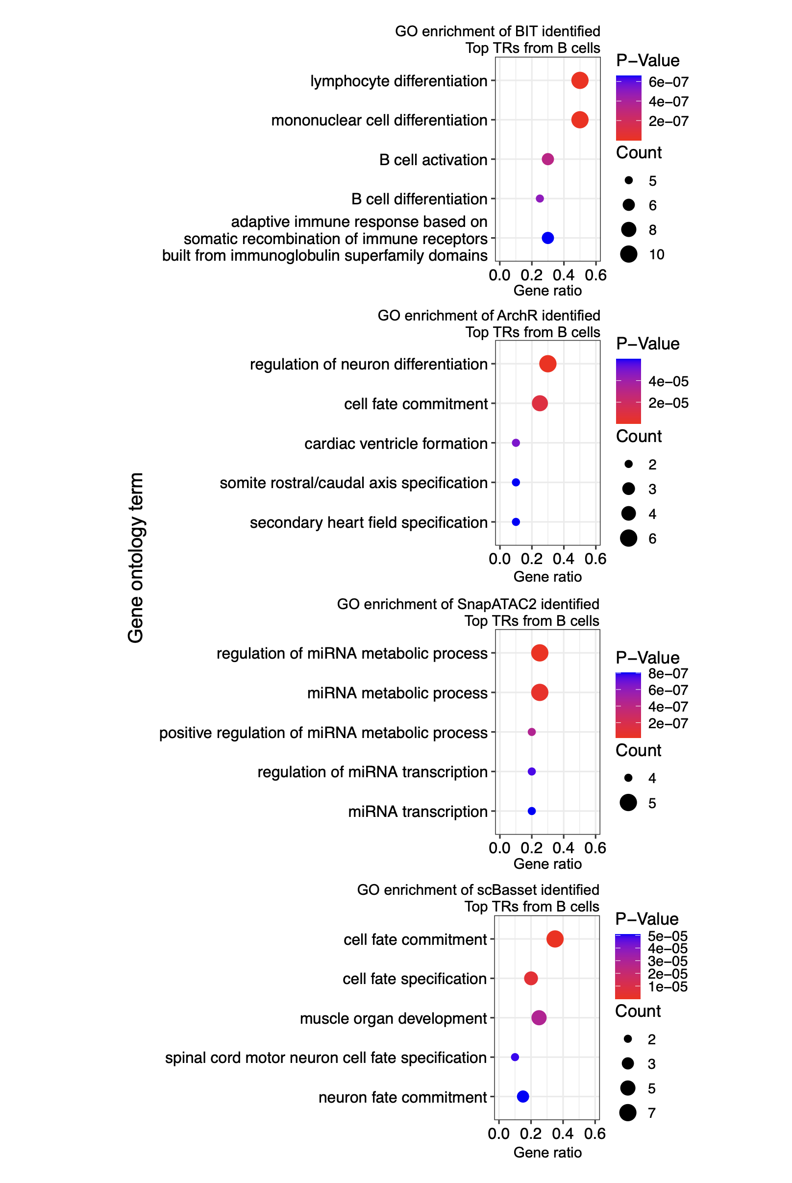
We plot the GO enrichment analysis results of top TRs by each method:

# -----------------------------
# Define Working Directories
# -----------------------------
# Main working directory
work_dir <- "/Users/zeyulu/Desktop/Project/BIT/revision_data/comparison/"

# -----------------------------
# Read In Results from Different Methods
# -----------------------------
# Read BIT and ArchR results (set first column as row names)
BIT_result <- read.csv(paste0(work_dir, "BIT.csv"), row.names = 1)
ArchR_result <- read.csv(paste0(work_dir, "ArchR.csv"), row.names = 1)

# For ArchR results, remove additional annotations by splitting at '_' and keeping the first part for each column
for (i in 1:9) {
  ArchR_result[, i] <- sapply(strsplit(ArchR_result[, i], "_", fixed = TRUE), function(x) { return(x[[1]]) })
}

# Read scBasset results and select every other column (columns 1, 3, ..., 17)
scbasset_result <- read.csv(paste0(work_dir, "scbasset.csv"))
scbasset_result <- scbasset_result[, c(seq(1, 18, 2))]

# Read SnapATAC2 results (set first column as row names)
SnapATAC2_result <- read.csv(paste0(work_dir, "SnapATAC2.csv"), row.names = 1)

# -----------------------------
# Define Common Cell Type Names and Rename Columns
# -----------------------------
# List of cell types to use as column names for each method's result
Cell_Types <- c("B cell", "CD4+ cell", "CD8+ cell", "Dendritic cell", "gdT cell", "HSPC", "MAIT cell", "Monocyte", "NK cell")

# Assign cell type names to the result data frames
colnames(BIT_result) <- Cell_Types
colnames(ArchR_result) <- Cell_Types
colnames(scbasset_result) <- Cell_Types
colnames(SnapATAC2_result) <- Cell_Types

# -----------------------------
# Extract Top 20 Genes for "B cell" from Each Method
# -----------------------------
# Create a list containing the top 20 genes for B cell from each method
Top20_list <- list(
  "BIT" = BIT_result$`B cell`[1:20],
  "ArchR" = ArchR_result$`B cell`[1:20],
  "scBasset" = scbasset_result$`B cell`[1:20],
  "SnapATAC2" = SnapATAC2_result$`B cell`[1:20]
)

# Display the Top20_list
Top20_list

# -----------------------------
# Perform GO Enrichment and Plotting for Each Method
# -----------------------------
# Loop over each method in the Top20_list (4 methods)
for (i in 1:4) {
  # Convert gene symbols to ENTREZ IDs using the 'bitr' function
  BIT_gene_ids <- bitr(Top20_list[[i]], fromType = "SYMBOL", toType = "ENTREZID", OrgDb = "org.Hs.eg.db")

  # Perform Gene Ontology enrichment analysis on the converted ENTREZ IDs (only considering Biological Process: BP)
  BIT_Results <- enrichGO(
    gene          = BIT_gene_ids$ENTREZID[1:20],
    OrgDb         = "org.Hs.eg.db",
    ont           = "BP",
    pAdjustMethod = "BH",
    pvalueCutoff  = 0.01,
    qvalueCutoff  = 0.05
  )

  # Extract the top 5 GO terms from the enrichment results
  GO_BIT_table <- head(BIT_Results, 5)

  # Create a data frame for plotting with columns for GO term description, gene ratio, p-value, and count
  GO_PLOT_Table_BIT <- data.frame(
    GO = GO_BIT_table$Description,
    GeneRatio = Trans_to_double(GO_BIT_table),  # Custom function to transform gene ratio values
    Pvalue = GO_BIT_table$pvalue,
    Count = GO_BIT_table$Count
  )

  # Generate a ggplot for the GO enrichment results
  plot_list[[i]] <- ggplot(GO_PLOT_Table_BIT, aes(x = GeneRatio, y = reorder(GO, -Pvalue), size = Count, color = Pvalue)) +
    geom_point() +
    # Customize the color scale for P-values with 4 pretty breaks
    scale_color_gradient(
      low = "red",
      high = "blue",
      limits = c(min(GO_BIT_table$pvalue), max(GO_BIT_table$pvalue)),
      breaks = scales::breaks_pretty(n = 4),
      guide = guide_colorbar(
        order = 1,
        title.position = "top",
        barheight = unit(1.6, "cm"),
        ticks = FALSE
      )
    ) +
    # Customize the size scale for Count with integer breaks
    scale_size_continuous(
      breaks = integer_breaks(GO_PLOT_Table_BIT$Count, n = 4),
      range = c(2, 5),
      guide = guide_legend(
        order = 2,
        title.position = "top",
        override.aes = list(color = "black")
      )
    ) +
    theme_bw() +
    labs(y = "GO", x = "Gene Ratio", color = "P-Value", size = "Count") +
    theme(
      text = element_text(size = 12),
      legend.position = "right",
      legend.box = "vertical",
      legend.spacing.y = unit(0.1, "cm"),
      legend.margin = margin(0, 0, 0, 0),
      axis.text.y = element_text(color = "black")
    ) +
    xlim(c(0.0, 0.6))
}

# -----------------------------
# Combine and Display Plots
# -----------------------------
# Combine the four individual plots into one layout with 2 columns and shared axis titles
p_combined <- plot_list[[1]] + plot_list[[2]] + plot_list[[3]] + plot_list[[4]] +
  plot_layout(ncol = 1, axis_titles = "collect")

# Print the combined plot to display the GO enrichment results for each method
print(p_combined)